Reinforcement Learning Course 1 Week 4

Notes for Reinforcement Learning Course 1 Week 4.

TLDR

• Evaluate the policy: How good is the policy?
• Update the policy: Let’s improve our actions!
• Dynamic Programming in the context of Reinforcement learning

Prerequisites

Previous blog, Reinforcement Learning Course 1, Week 3

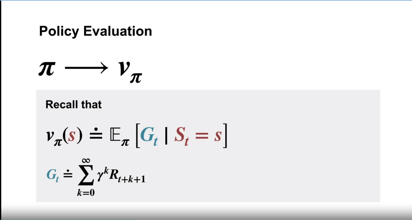
Policy Evaluation

From the previous blog, we learned about a state’s value. We can denote this as $v(s)$. Now, the value of a state will depend on two things. One is how easily we can get the maximum reward from the state. Two is what action we will take, i.e., what policy we will follow in that state! We can denote it as $v_{\pi}(s)$. Which means the “value of a state while following the policy $\pi$.”

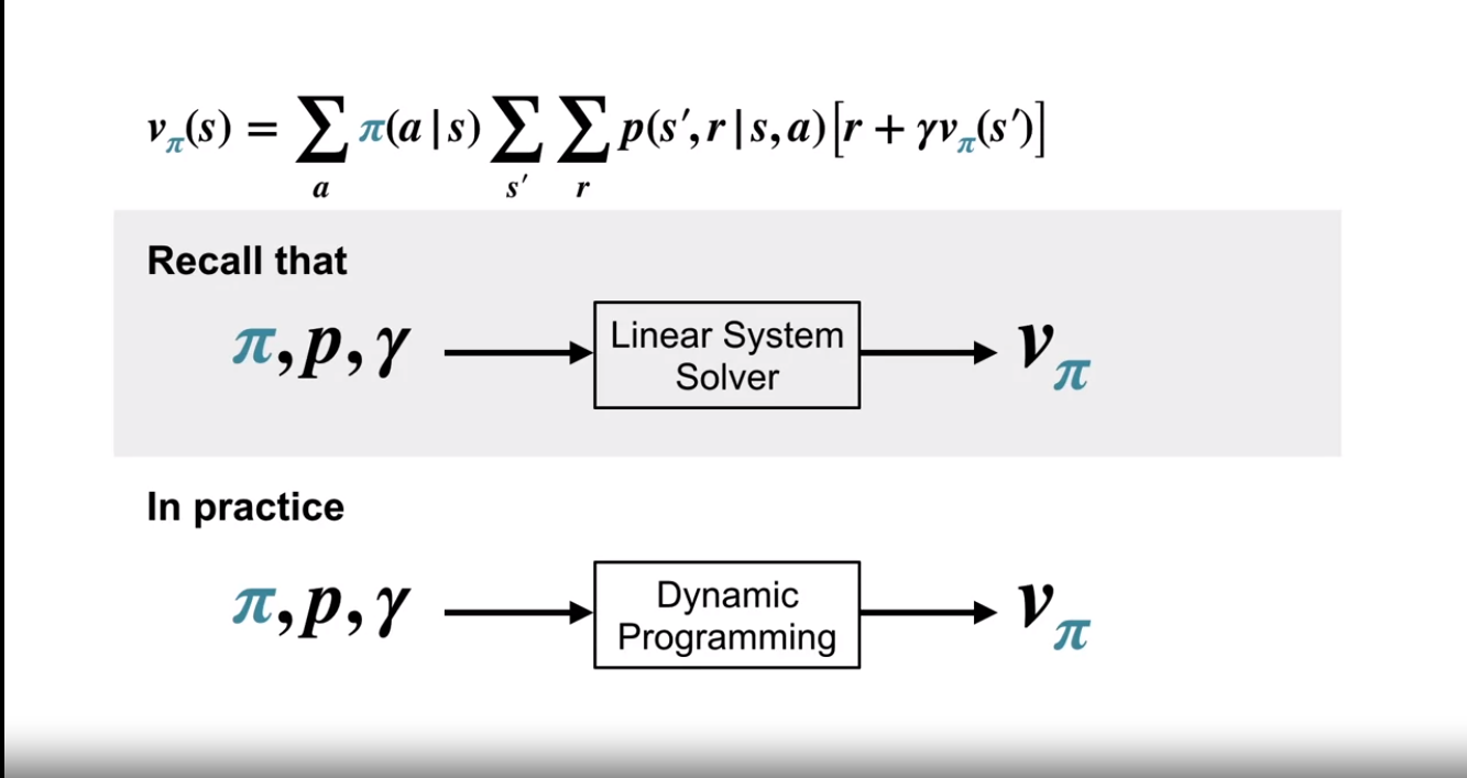
From the first blog, we can recall $ \begin{equation} v_{\pi} (s) = \displaystyle\sum_a \pi(a|s) \displaystyle\sum_{s’}\displaystyle\sum_r p(s’, r|s, a)[r + \gamma v_{\pi} (s’)] \end{equation} $

For each state, we will get a different equation. From the equations, we should be able to solve and get the optimum value $v_{\pi}$! But the problem is that in practice, the states are often continuous! That means infinite states, and hence, infinite equations are possible! Not to mention, for different policies, $\pi$, the equations will change! So what do we do? We go for an iterative solution! We use dynamic programming algorithms (yeah, that dynamic programming is used in problem-solving!).

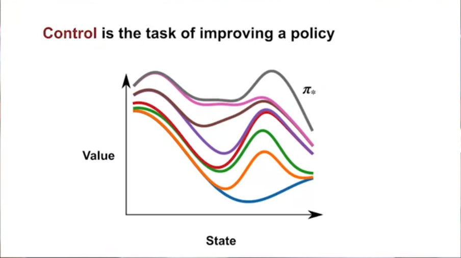
Control

Control in this domain means improving the policy. How do we know which policy is better? Simple! The policy for which the value of the same states is greater! If the $v_{\pi2}$ for all states are greater than $v_{\pi1}$ , then we can tell $\pi_1$ is better than $\pi_2$ ! What if the police values are not greater but equal to all of the previous policies? We can assume that we have converged to the optimal policy!

Note there is a mention of “strictly” better policy; I am not sure what that means. I will check in the book to get a better idea!

How will we use Dynamic Programming?

Well, to be honest, it will become clearer as the course progresses, and hence this blog! But in short, dynamic programming will be used to approximate the optimal value and the optimal model of the environment to get the optimal policy! More on that later!

Iterative Policy Evaluation

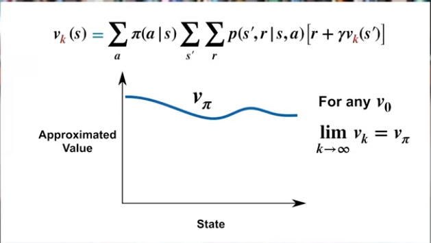
What is the Iterative policy evaluation? Simple. We have the bellman equation at (1), correct? Suppose we have an initial random policy value $v_k$. What if we tug the value into the (1)? $ \begin{equation} v_{k+1} (s) = \displaystyle\sum_a \pi(a|s) \displaystyle\sum_{s’}\displaystyle\sum_r p(s’, r|s, a)[r + \gamma v_k (s’)] \end{equation} $

What does it mean? Using the Bellman equation, we got better at estimating the optimum value function!! If we do this overall state-specific “iterations,” we should get the optimum value function!! When do we know the value function has reached the optimal value? When the value functions are not changing! Because the $v_{\pi}$ has only one unique solution to the bellman equation.

Intuition

Note: It seems that the $v_k$ is improving iteratively; need some proving which was not given by the video

I have an intuition!

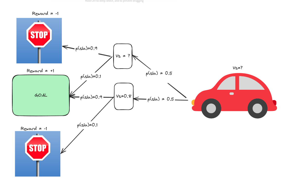
Suppose you are in a car that moves randomly (hopefully you DO NOT drive such cars!). The probability distribution and rewards are as follows,

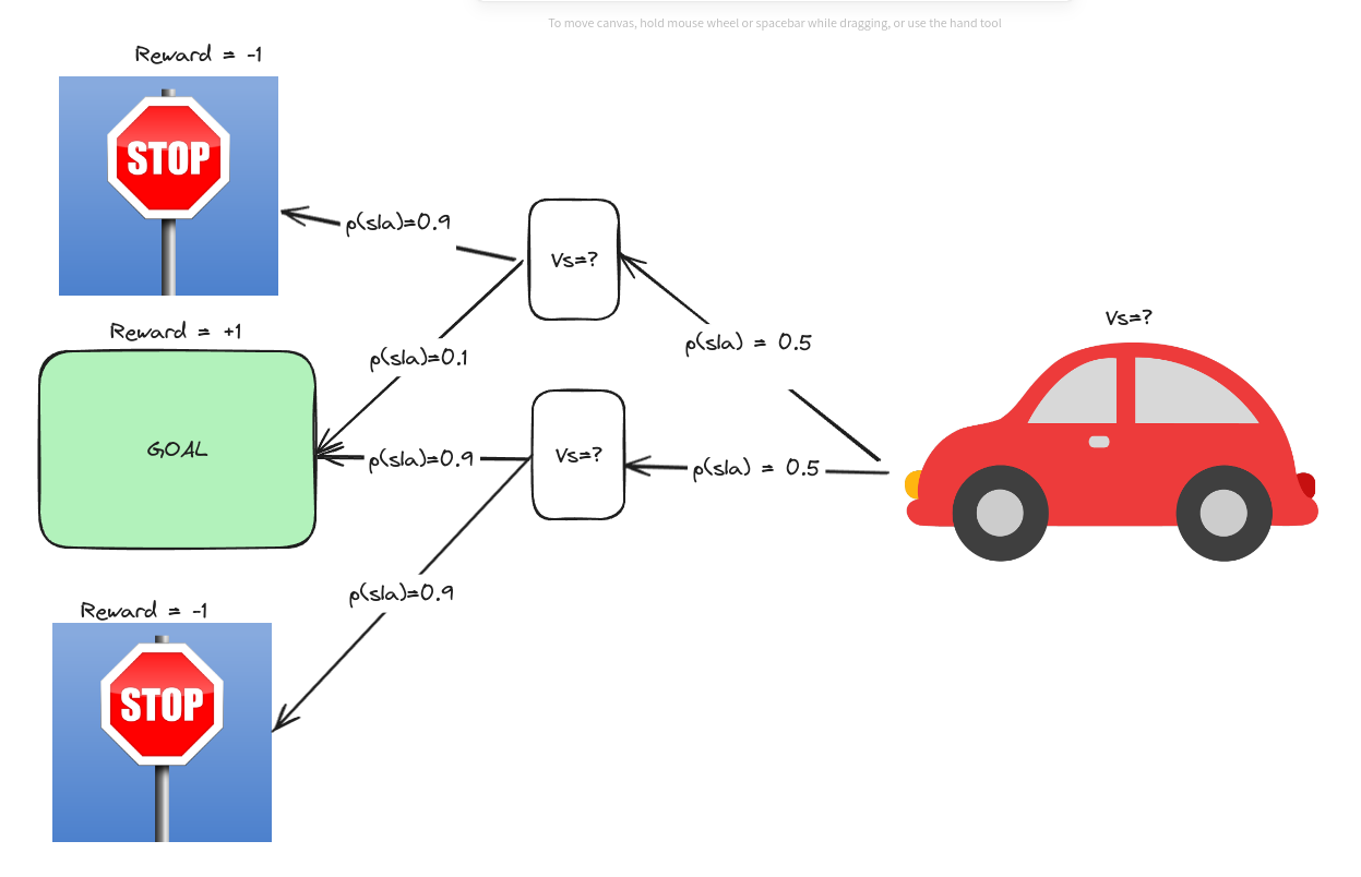
That means, given the state, the car has a 50% chance of moving to the upper or lower state. If it reaches the upper state, then according to the diagram, it will have a 90% probability of reaching the state with a reward of $-1$. But if it reaches the lower state, it has a 90% probability of reaching the state with a reward of $1$. In that case, for the upper state, we can calculate the value $v_s$

Using the equation above

reward $r=0$, final state value is the reward $-1$ or $1$

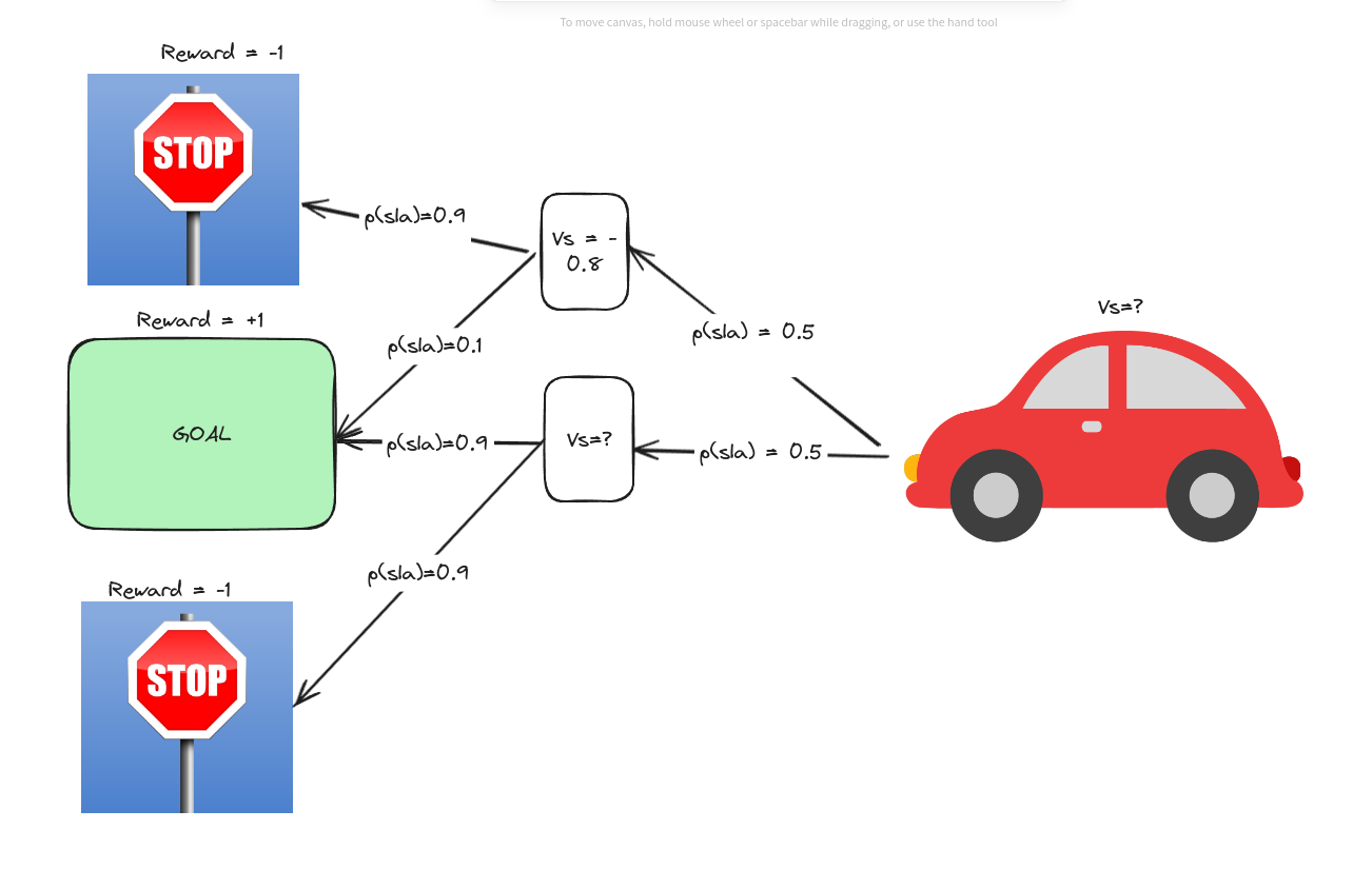
$v_s = 0.9 * (0 + (-1)) + 0.1 * (0 + 1)$

or, $v_s = -0.8$

We can calculate the same value for the lower state.

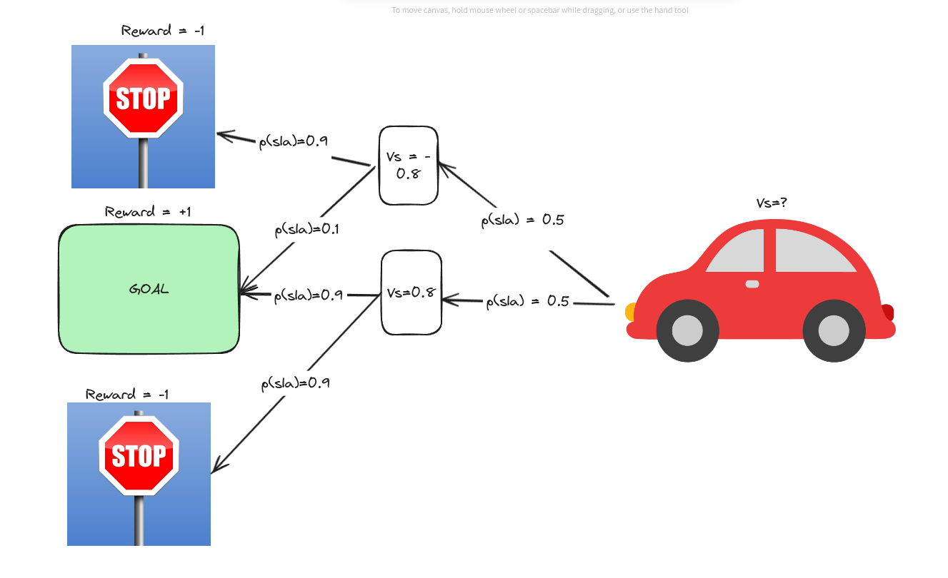
Now, we do not know the initial state value. From the same process, we can get the initial state value,

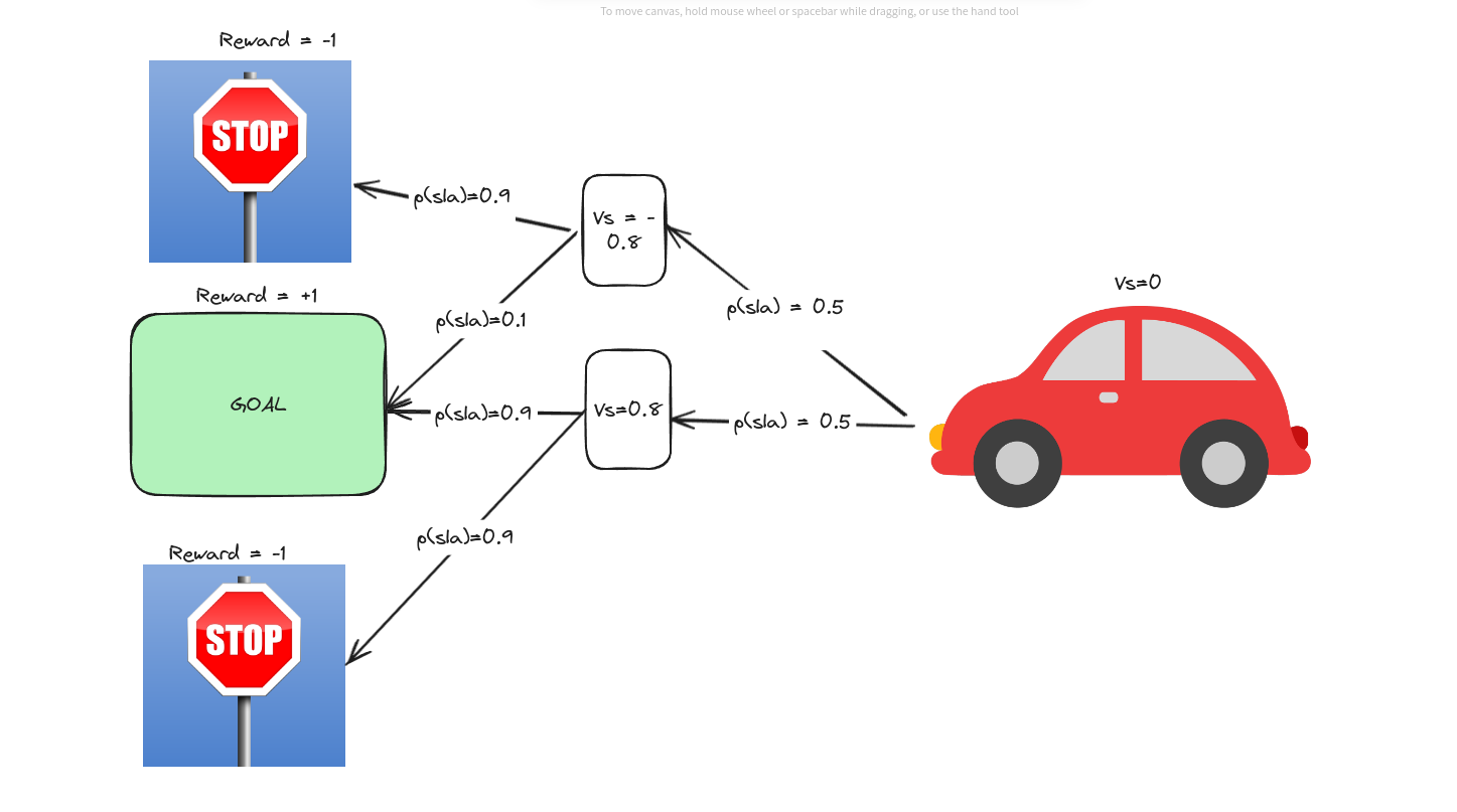
It seems $vs=0$! Does it mean no value? Yes! Because, by being on the initial state ONLY, there IS NO BENEFIT! As the process is entirely random!!!

I hope the intuition helps the readers understand the bellman equation better!

Policy Improvement

Now, you’ve had enough of randomly selecting a car! Now you know the value of each state, so you decided to do something! What did you do? You went to the next state with a higher value than yours! That is the point of value, isn’t it?!

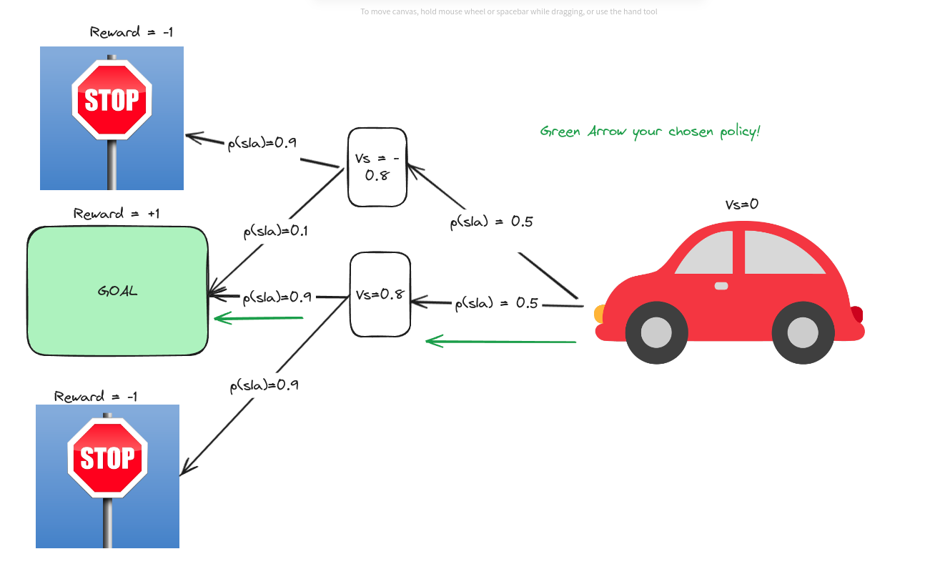
In that case, you go to the goal state pretty quickly!!! That’s pretty common sense,

So because you just went to the States with a higher value than yours, we can say you were “greedy.” This kind of thinking, to change the policy $\pi$ into $\pi ‘$, is called Greedy Policy. Because you are greedy, after all! The idea of the policy improvement theorem is that,

suppose you have value $q(s, \pi(s))$ for all states $s$ . Then, at the next iteration, you choose new policy $\pi ‘(s)$, which is to choose the action with highest value $q(s, \pi(s))$, then $\pi ‘$ must better or at least equal to the $\pi(s)$! In mathematical terms

$\begin{equation} \pi ‘ (s) = \displaystyle\argmax_{a} \displaystyle\sum_{s’}\displaystyle\sum_r p(s’ , r |s, a)[r + \gamma v_{\pi}(s’)] \end{equation} $

$\begin{equation} \implies \pi ‘ >= \pi \end{equation}$

Policy Iteration

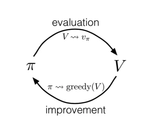
The equation $(3)$ shows that the greedy policy should be better than the policy on which the value function is calculated. Suppose for policy $\pi_1$, we get value $v(\pi_1)$. Based on the $v(\pi_1)$ , we get greedy policy $\pi_2$ . Something like the following,

$ \pi_1 \rightarrow v(\pi_1) \rightarrow \pi_2 \rightarrow v(\pi_2) \rightarrow ….\pi^* $

Whereas $\pi^*$ is the optimal policy.

We can see a loop going on here,

What if the initial policy needs to be better?

This is a personal note: In the more complex problems, the initial policy also dictates whether we can truly reach the optimal policy or not! These issues will come in later blogs!

Generalized Policy Interaction

From the above car example, we used the equation (2).

$v_{k+1} (s) = \displaystyle\sum_a \pi(a

s) \displaystyle\sum_{s’}\displaystyle\sum_r p(s’, r

s, a)[r + \gamma v_k (s’)]$

We calculated the value for every probable action from a given state. In the end, we only took the “greedy” option. What if, while calculating the value of a state, we only calculated the value for the action with the maximum next value? Then, within one pass, we would get the value.

then, we can also get the value of the initial state,

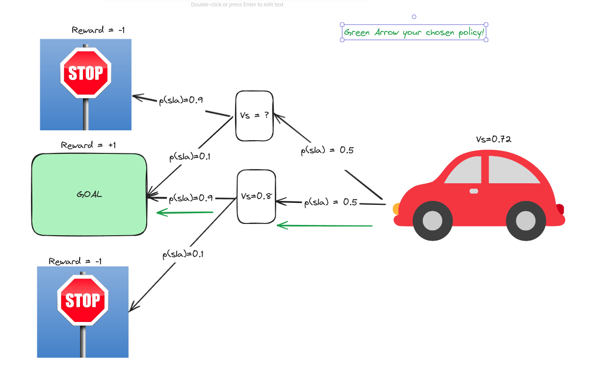
This took only two steps! We can call this the General Policy Iteration framework.

Now, the equation becomes

$\begin{equation} v_{k+1} (s) = max_a\displaystyle\sum_{s’}\displaystyle\sum_r p(s’, r|s, a)[r + \gamma v_k (s’)] \end{equation}$

Because we are not checking the policy evaluation directly in this case, we call this method Value Iteration.

Dynamic Programming Efficiency

The way we approached the Belman equation is part of dynamic programming. To better understand dynamic programming, please check this video.

The model of the environment is known in the examples of this blog and the course. As it is known, we can use dynamic programming to iteratively get the values of the states. But are there other methods? If yes, which is the best approach?

There are other approaches.

• Monte Carlo approach. I do not know why they named it in such a way (maybe some reader can point it out.) In this approach, we do not use all of the states. We take samples of the states, actions, rewards, and actions in the following states, then use the updated Bellman equation to get the values of the states.

$\begin{equation}V(s) = \frac{\displaystyle\sum_{t=1}^T[S_t=s]G_t}{\displaystyle\sum_{t=1}^T[S_t=s]}\end{equation}$

That means we take the samples and get the average of the expected return values. However, this has a big margin of error as it only calculates certain samples.

• Brute-Force Approach: As the name suggests, here we calculate the Values of all states for all actions possible. But this will become highly inefficient as even for small environments (i.e., where the number of states is few), the number of state action pairs can rise exponentially!

That is why the dynamic programming approach is the best. But here is a caveat! We assumed we know the model dynamics! What if we do not?!! We can explain those in later chapters!

Reference

[1] All of the images on the equations are screenshots from the Course video.

[2] The equation 6 is from the lilianweng blog

[3] The Intuition on the Policy Iteration with the car is drawn in Excalidraw.