Reinforcement Learning Course 1 Week 2
Notes for Reinforcement Learning Course 1 Week 2.
TLDR
- Introduction to MDP
- Dynamics of MDP
- Continuous Tasks
- Discounting
Prerequisites
To start reading this blog, please read the first blog of the series, Reinforcement learning specialization, Course 1, week 1.
K-armed bandit into Markov Decision Process
Problems of K-armed bandit world.
-
In the K-armed bandit problem, all actions are the same. For example in a medical trial, we choose medicine from one of the three. We do not choose, medicine at one time, and exercise in the other situation, for example. In the real world, we need to choose different actions for different situations.
-
Another issue with the K-armed bandit problem does not consider the long-term consequences. For example, a patient may heal right away for medicine A compared to that of medicine B, but it might have some other lifetime side effects. The K-armed bandit problem does not consider that.
Then what does the real world more like?
In the real world, we interact with the environment, we get some feedback (it might be positive/ negative or neutral). Then based on the new state we take new actions! Something like this,
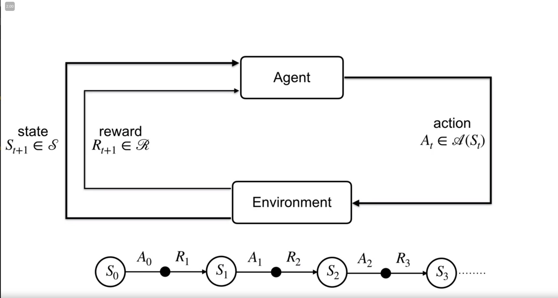
where,
$S_t$ : State at time $t$. $S_{t+1}$: State after action $A_t$ at time $t+1$
This cycle of $(state, action, new state, reward)$ is known as Markov Decision Process (MDP in short).
Representation of MDP
The mathematical representation of the MDP is as follows
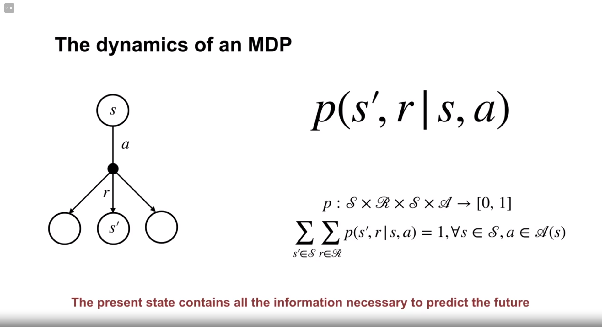
In the above haunted (!) mathematical picture the terms mean as follows,
| $p(s’, r | s, a)$: It means the probability of a new state and reward given the current state $s$, and action $a$. |
We assume the environment is stochastic, and hence it is shown as a probability function. Because of that, the summation of probabilities, across all rewards and states is $1$.
Real Life Intuition
We can express any real-life events or cycles of events as MDP. This is the flexibility power of the MDP framework. For example, 5 days-a-week work life. Let’s assume the following,
- Your energy level is the state $s$
- Your commute to work, coming back home, and working at the office all are action $a$.
- For each action, we have state transition probability $p_a$.
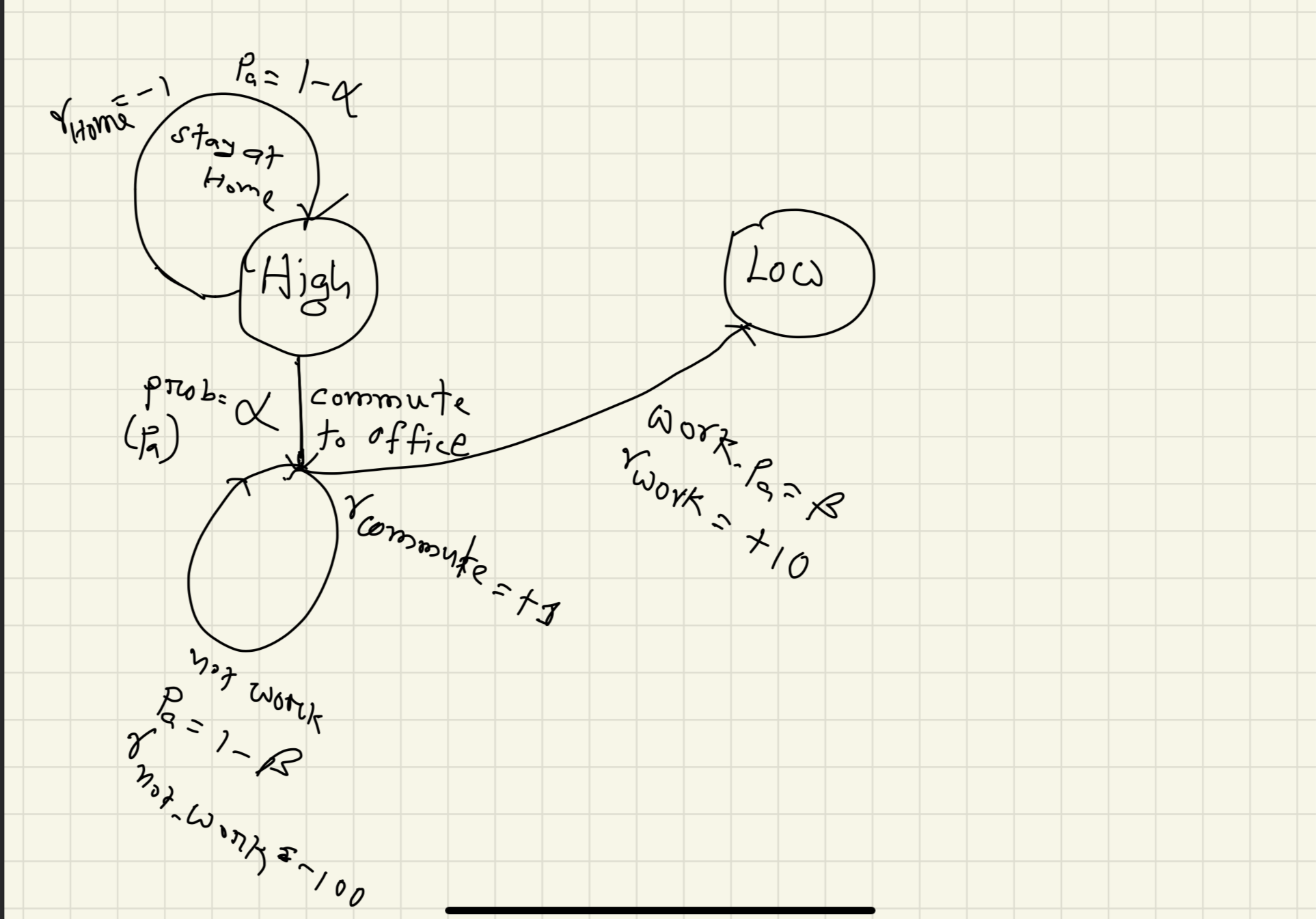
Let me first show you a scarry final diagram, 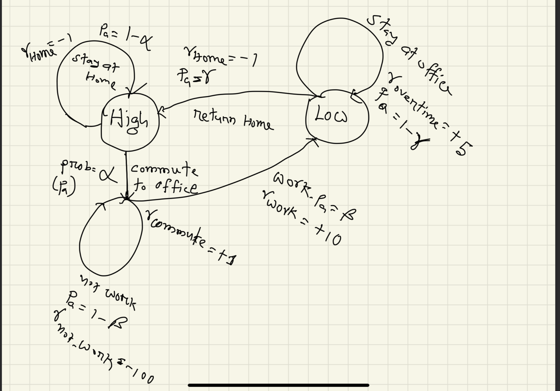
How did we get here?
From the beginning, your energy level is either high or low. Which are the states?
In the morning you (hopefully) wake up and commute to work.
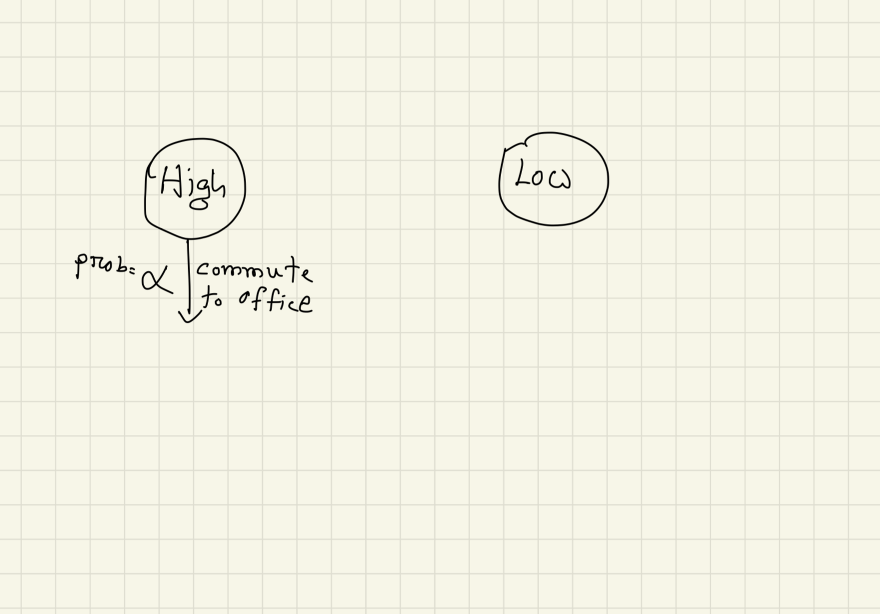
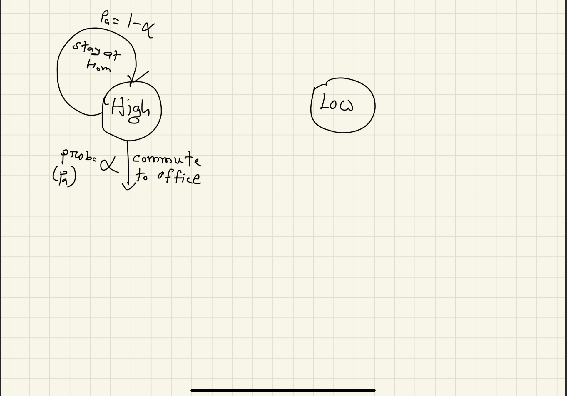
The world is not deterministic my friend! “Probably” you will go to work, or probably not! So let us give this going to work a probability, $p_a= \alpha$. So, if you somehow stay at home, that would have probability, $(1-\alpha)$!
 .
.
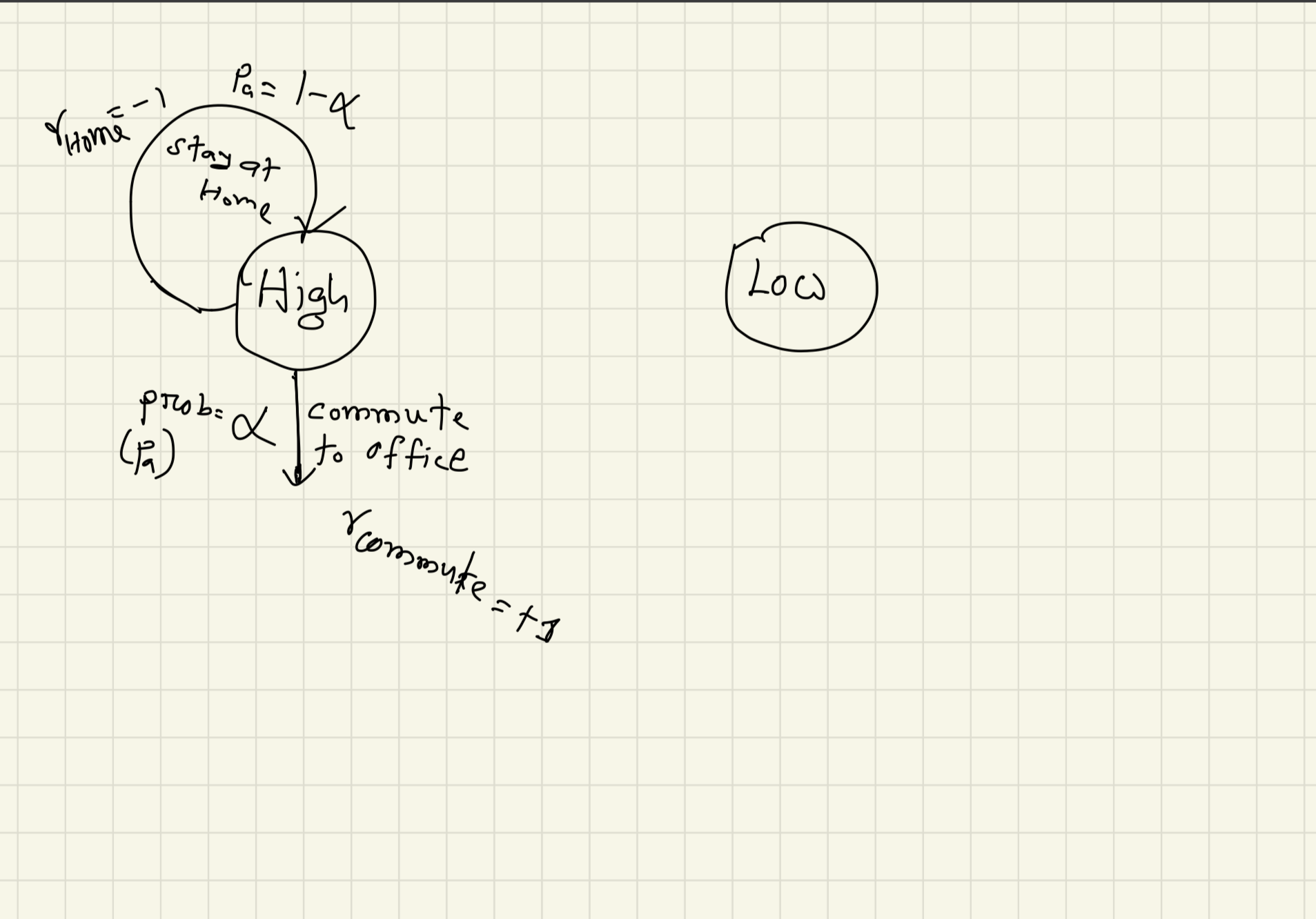
If you stay at home, you will get some negative feedback from the office! Let us say, you will get, a reward $r=-1$. If you go to the office, you will get a reward of $r=+1$.
Again, you may work at the office, or waste your time! Let us say you work at the office with the probability $p_a=\beta$. You will get a reward of $10$. But because of that, your energy will decrease!
 .
.
After you finish your work, you get back home. But you may not! If you get back home with the probability of $\gamma$, you will get the negative reward (because your company likes “Hard-working” people who overtime!) of $r=-1$.
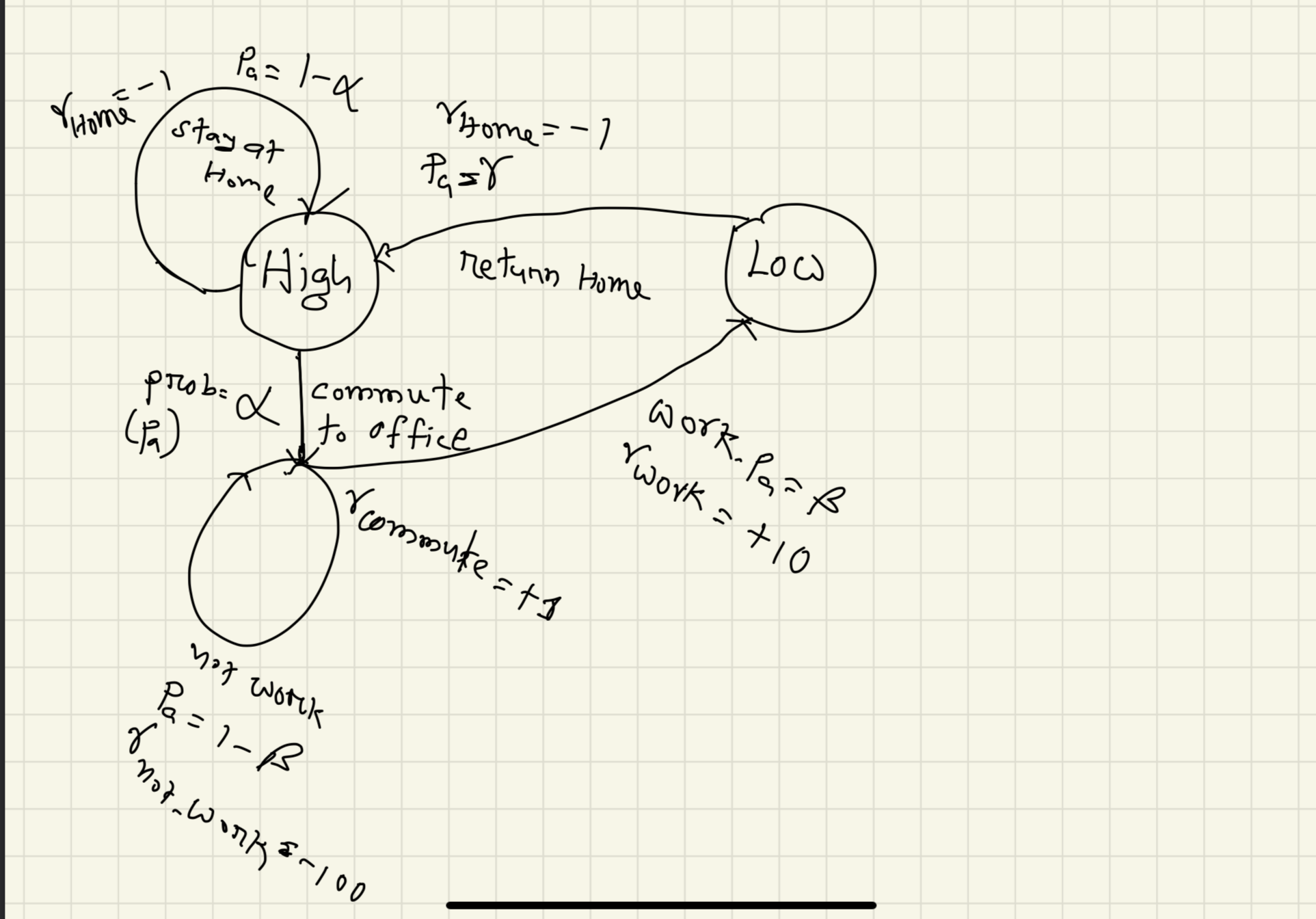
But if you stay late (with the probability of $1-\gamma$), and work overtime? You get a reward, $r=+5$.
What do we see from the above plots?
The power of Markov Decision Process lies in that, we can convert any situation into a pair of $state, action, probability, reward$!! This helps us formalize any problem anywhere!
Goal of the Reinforcement Learning
In one sentence, the goal of the reinforcement learning is to maximize the future rewards. What do we mean by that?
Well, in the above example of MDP, if we always prioritize the immediate reward, what will happen? If we are asleep to keep our energy high, one day we will run out of money and we will starve! If we keep working to get rewards from the companies, we will lose our personal lives, families, and energy! So what do we need? Maximizing the future rewards! We need both work and personal lives to have the best of all worlds! This is always the goal of any RL agent!!
The reward Hypothesis
This video is very important about the philosophy behind Reinforcement learning. The video is craftfully presented by Michael Littman. The basic idea of Reinforcement learning is that we do not teach the agent the exact actions. Rather we feed them the rewards for a certain action at a certain state. From this information, the agents should learn the correct actions to maximize the total or cumulative rewards.
Now this idea has an assumption. That is, the environment is giving us back the correct rewards. But in real life do we get the correct rewards? Or, how can we define the correct rewards? For stock market problems, we can easily set the monetary value as a reward. When you buy stocks you lose money, when you profit, you gain money! There is a “common currency”! But what about thermostats in the AC? How can you measure your comfort zone and the energy cost of achieving it? No common currency!
We can set the goals as rewards. If you take a step, you get a $-1$ reward, when you receive the goal, you stop getting negative rewards. This is known as action-penalty representation. Otherwise, you achieve 0 for any action and 1 for the goal. This is known as goal-reward representation. But there are some problems with this. The first one has a problem of getting stuck somewhere without reaching the goal. The second one does not create any urgency for the agent! Both have a problem if the goal is after a really long sequence of actions!
For example, if you give the agent +1 for achieving the Nobel prize and 0 otherwise, the agent will not have enough information to go in the right direction at all!
How to define rewards
Programming is the most common way to define the rewards. Sit down understand the dynamics of the environment, and then define the rewards. Another research is the use of temporal logic.
Another interesting way is getting rewards from human beings. This is known as human-in-the-loop. In this case, the human beings will be like guides to the agents. The best example is RLHF, reinforcement learning with human feedback used in ChatGPT.
The other way is to mimic rewards from another agent (likely human beings). The most interesting application is Inverse reinforcement learning. Where the agent learns the rewards based on behaviors.
The other ways mentioned are Evolutionary optimization, Meta RL, etc. upto 9:30
Challenges to the Hypothesis
-
How to represent risk-sensitive behavior? The behaviors which may be best to maximize your total rewards, but also cause you risk? [Example?]
-
How about some diversity in behavior? A classic example is the music recommendation. No matter how much you like a song, listening to it repetitively will make it boring! The reward hypothesis does not endorse the diversity unless we can tweak the system for some exploration!
-
Another problem is, can we model human behavior solely on maximizing rewards? For example, if you cheat in an exam, you will get high rewards, but cheating is bad! The reward hypothesis does not consider how you get the maximum reward! But humans do have ethical issues outside of the reward hypothesis!
Anyway, these challenges to the reward hypothesis lead us to future research on Reinforcement learning!
Episodic Tasks and Continuing Tasks
Till now, all the discussions were related to the tasks or works assuming the task will end once! What if it doesn’t? For example, if we are playing a game of football - some call it soccer - the game will end after 90 minutes assuming no extra time. These kinds of tasks are known as episodic tasks. What if it is a Badminton match? There is no time bound! Only when one player can score 21 points, the game is over! This can be summarized as a type of Continuous task! Or suppose from a real-world example, Refrigerator. The refrigerator is always on! Continuous task!
Wait, what about total rewards?
For Episodic tasks, the total rewards are finite.
$G_t = R_t + R_{t+1} + R_{t+2} + R_{t+3} + ……R_n$
But for the continuous tasks?
$G_t = R_t + R_{t+1} + R_{t+2} + R_{t+3} + ….$
The total rewards seem to be infinite?!! We have a solution for that!
Discounting
We rewrite the equation for the continuous tasks as
$G_t = R_t + {\gamma}R_{t+1} + {\gamma}^2R_{t+2} + ……$
The coefficient ${\gamma}$ is known as the discount factor whereas $0 < \gamma < 1$. What does it do? It signifies how much preference should be given to future rewards. In general, we want to give preference to the immediate rewards compared to the future rewards. You should care more about today’s food than the food you can eat after 30 years! If you do not eat today, you might not live up to 30 years!
Let’s see the equation,
$G_t = R_t + {\gamma}R_{t+1} + {\gamma}^2R_{t+2} + ……$
or
$G_t = R_t + {\gamma}{R_{t+1} + {\gamma}R_{t+2} + ……$
or
$G_t = R_t + {\gamma}G_{t+1}$
In other words, the expected rewards at time step $t$ can be equal to the sum of immediate reward and the expected rewards at time step $t+1$!
This equation can help us estimate the rewards for continuous tasks! This powerful equation will be exploited in the next notes!
Reference
- All of the screenshots are from Course 1, Week 2 of Reinforcement Learning Specialization.