Reinforcement Learning Course 1 Week 1

Notes for Reinforcement Learning Course 1 Week 1.

TLDR

• We get introduced to the K-armed bandit problem.
• Action values concept.
• Greedy actions.
• Epsilon greedy action selection, Optimistic Initial action values.
• Upper Confidence Bound Action selection.

Contact

• Email: sezan92[at]gmai[dot]com
• Linkedin: MD MUHAIMIN RAHMAN

Background

I am an RL enthusiast for a long time. The concept of training an agent based solely on the points fascinated me from the beginning! I kept exploring the RL methods and architectures by myself. For example, the blogs of The Game is ON! were based on my learning journey. It is still ongoing by the way!

But something was missing. I had some issues with the basic terminologies in the literature. Some of the important algorithms seemed very difficult to me. So I decided to step back and try to hone my basics! I tried to read The famous book by “Sutton and Barto”, but the book being a big Textbook, it also seemed very hard!

Somehow I got to know about the Reinforcement learning Specialization at the University of Alberta and everything changed! In this blog series, I want to share my thoughts/ideas/notes about what I learned from the specialization. I will try to explain in simple language. The specialization is really good. The first blog of this (hopefully) continuing blog series is about Course 1, Week 1 of the specialization. If there is any concern/question/feedback, please do not hesitate to email me at sezan92[at]gmail[dot]com.

Week 1

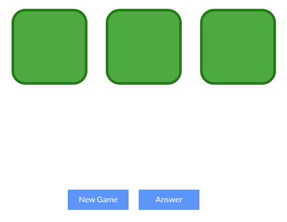
• In the first week, the instructors introduced the k-arm bandit problem. It is a simple game with multiple buttons. Each button will reward you. you need to choose the best button by pressing each button and maximizing the reward. The best similar thing is gambling!! But in our life, we may take decisions by trial and error.

  The game in the course looks like following

• On the example of K-armed bandits can be clinical trials

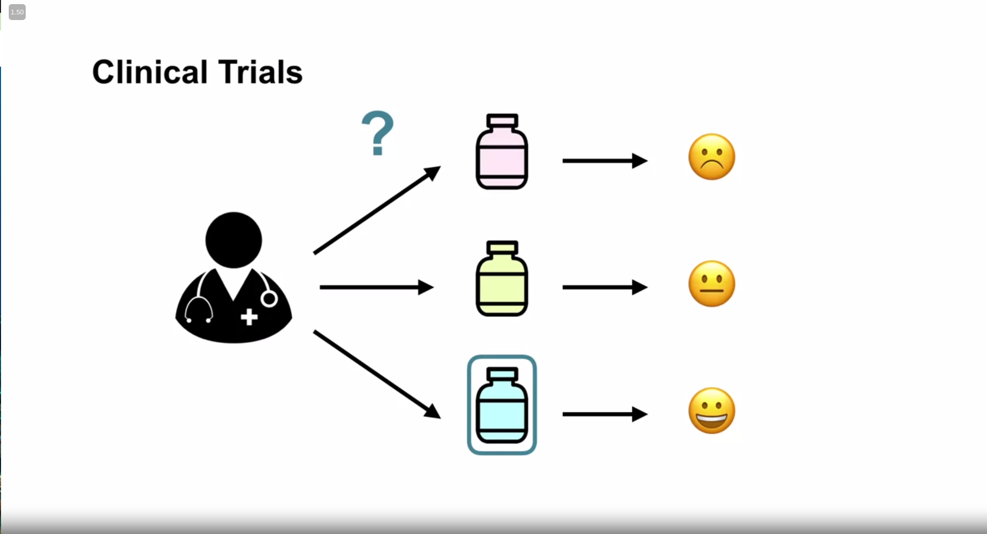
  The big idea is that suppose a doctor has 3 patients. he doesn’t know the medicine. so he trials 3 medicines for 3 patients. if he sees improvement in health in a patient for a certain medicine, he prescribes the medicine.

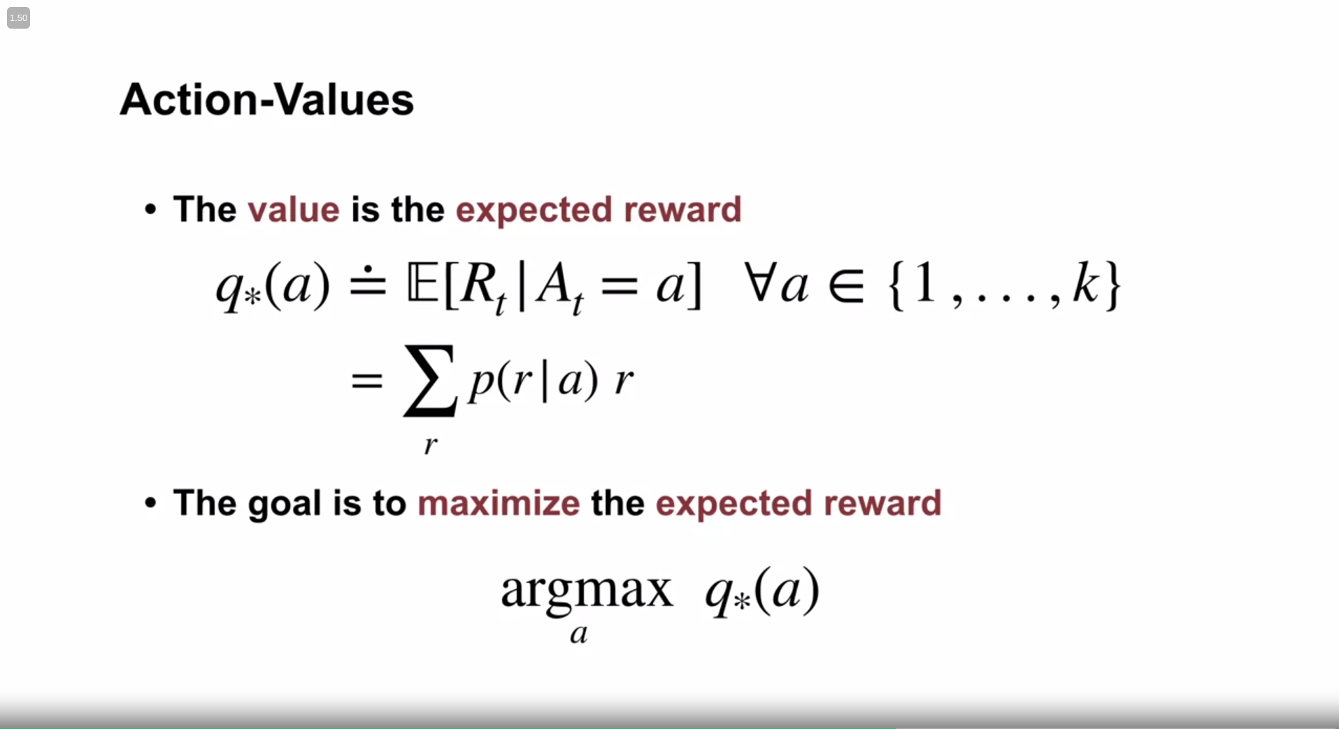
• Let’s define action and reward. The action is the prescription of a certain medicine and the value is the effects of the medicine. Progress can be seen as positive rewards, while regress can be seen as negative rewards. The combination of the both is Action value.

• For intuition, the instructor shares the following illustration

  

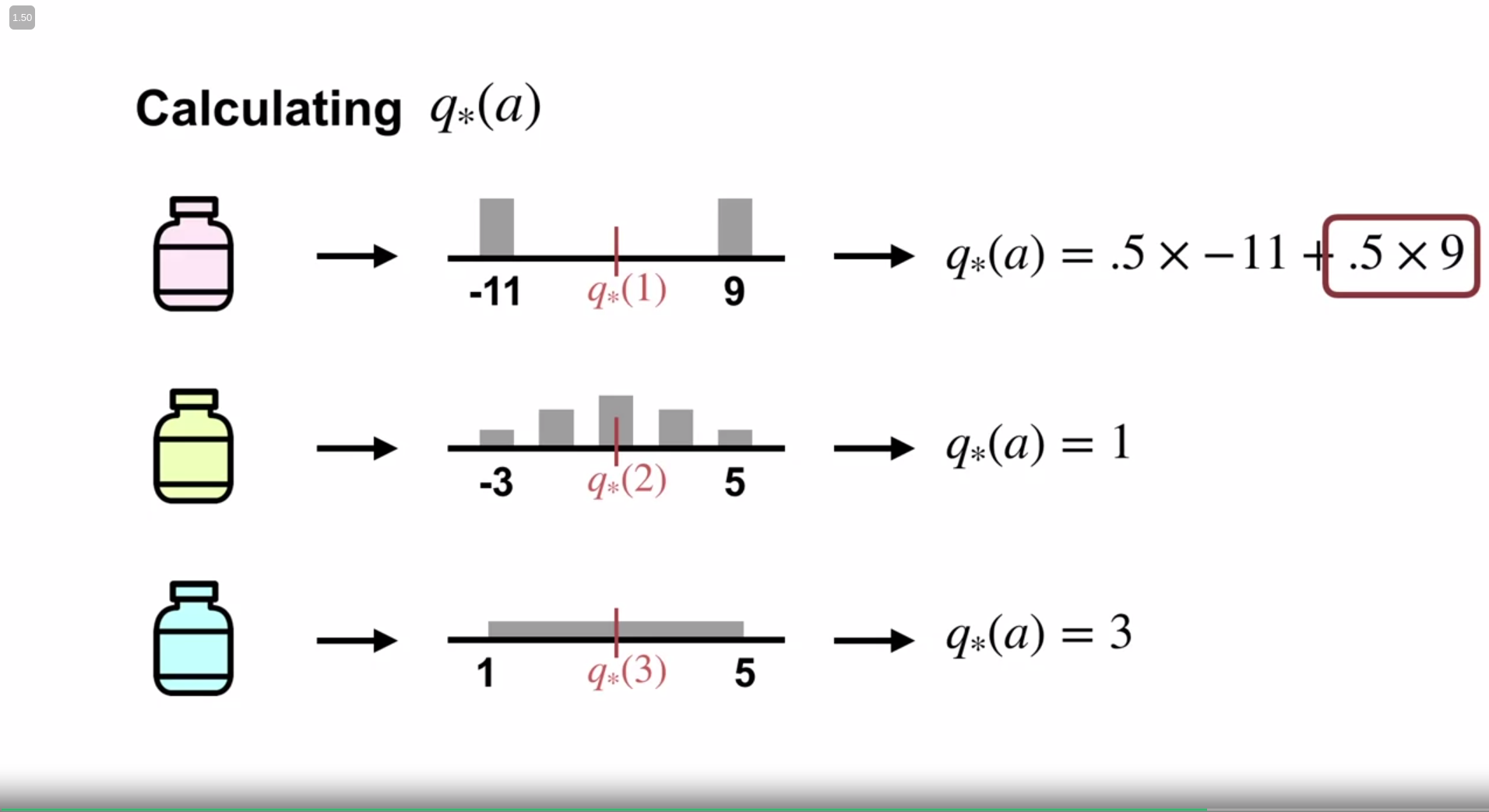
  Here, each action $a$ , (i.e. the prescribed medicine) has an action value $q(a)$ i.e. health state for that specific medicine.

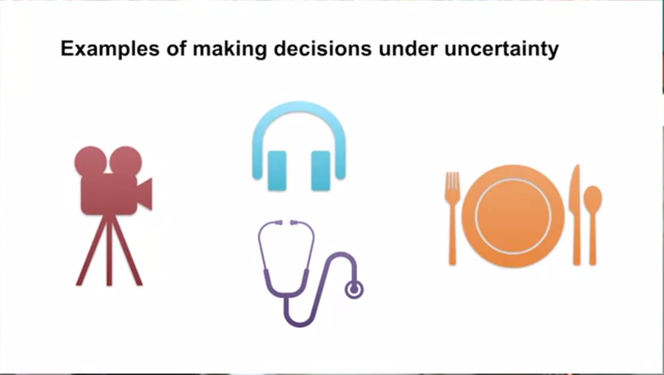
• Our real-life examples

• My comments: Although the given example is good for getting an intuitive understanding, it is not a concrete example. First of all, medical trials are not random trials. After many days of research, the doctors sort out some candidates to test, and then they make the study trials.

• The instructors could have gone with a simpler example, like which food is best in a country, which singer is the best etc.

Action value

Action value is the value of an action. (I know it is not genius to figure it out). But the question is how can we know the value of an action?

Referring to the example of intuition, how can we know the value of prescribing a certain medicine? One of the ways is the “Sample averaging method”.

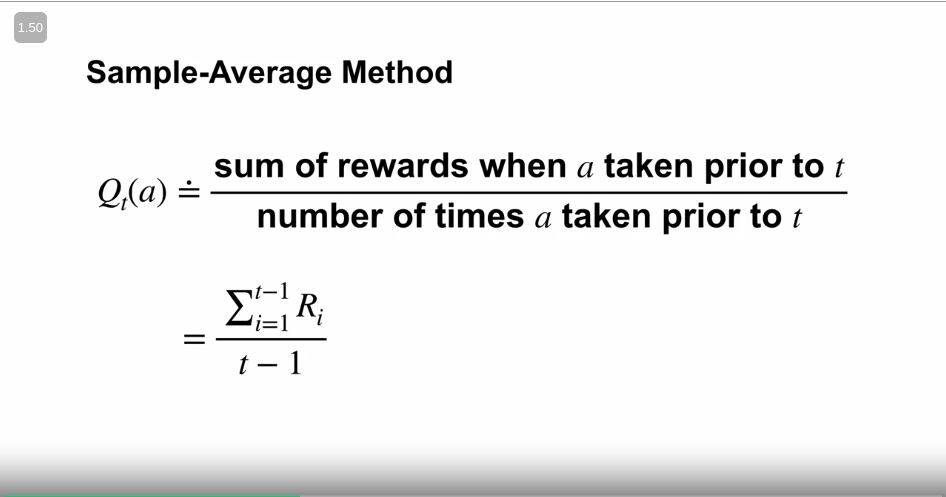
Intuition

For example, suppose the doctor decides again to do a random trial among headache pills $A$ and $B$. For medicine $A$ the headache is cured 90 out of 100 times, $B$ is 50 out of 100 times. We can conclude that the action value for $A$ is $90/100$ => $0.9$ . But what about the other 10? They might have other factors - which leads us to the notion of $state$ value- More on that later.

Greedy action

Suppose we get action values for all three actions after many trials. When we choose the action with the best action value, this is called greedy action selection. This process of choosing greedy action is known as exploitation.

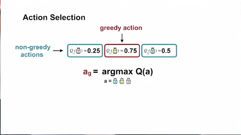
On the other hand, we also can explore other actions at the probable expense of getting the best reward. This will let us know more about the actions. We call this process -as one might have guessed- exploration.

Now, the problem is, we cannot do both at the same time. This is a fundamental problem in Reinforcement learning known as the Exploitation Exploration dilemma.

We can rewrite the sample-average method for learning action values as follows,

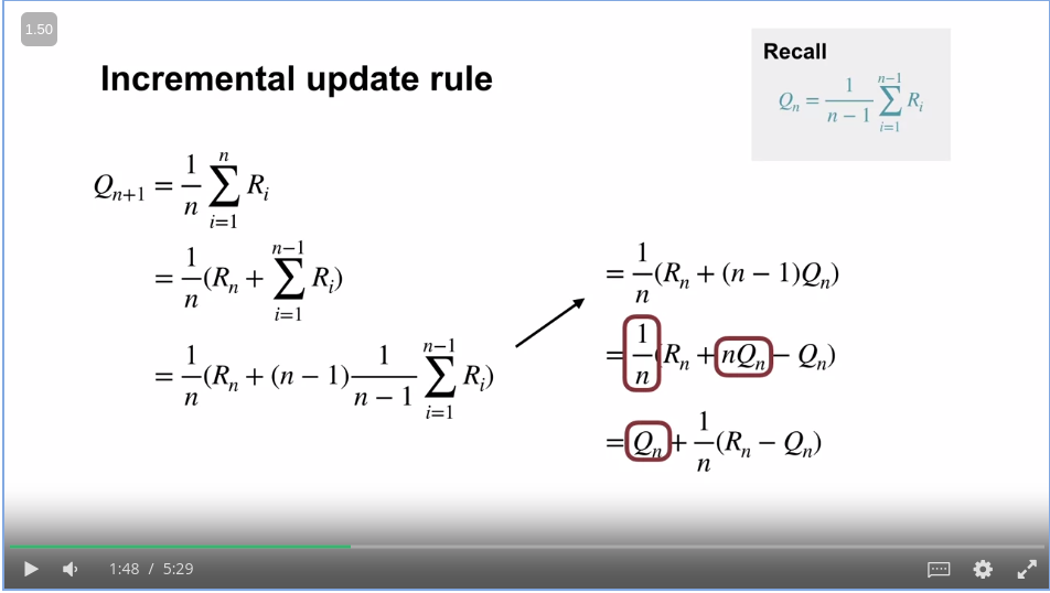
in other words,

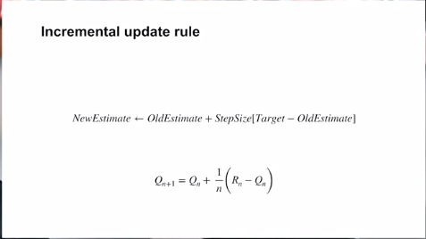
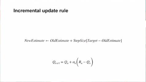
In the above equation, we can guess the term $\frac{1}{n}$ for a known number of steps. But what if we do not know how many steps will be taken? For example, we will never know how many moves a game of chess can be won. In those kinds of scenarios, we can write $\alpha$ instead! It is a hyperparameter known as step size which will dictate how quickly our agent can update the action value.

Non-stationary bandit problem

Let’s look at the equation again,

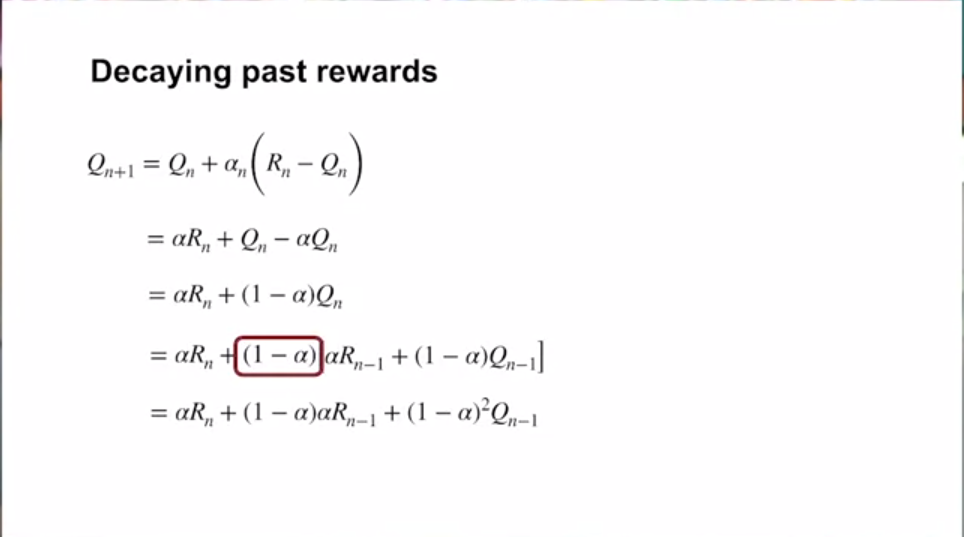
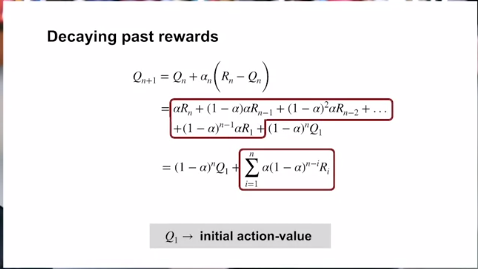
From the above two equations, we see that the term $Q_{n+1}$ depends on the most recent rewards more than the previous rewards. This is important!

It means that the Action values always give more focus on the recent rewards than the previous ones. Why is it important? It helps the model to be updated online! There might be some actions that might be time-dependent. e.g. some medicines might work in one season, but not in others seasons. This equation helps us keep track of recent rewards and let the model learn from the most recent experiences.

Exploration Exploitation trade-off

What is the trade-off?

Exploration means the agent tries each action and sees what the action leads to.

Exploitation, on the other hand, means that the agent takes action with the maximum rewards possible according to the most updated model.

Now, if we let the agent always explore, the agent will not ever act according to the latest pieces of information of best actions; resulting in never maximizing the total rewards! But if we always let it exploit, we might miss the information about all plausible state-action pairs! This is known as the exploration-exploitation dilemma.

Solution?

Epsilon Greedy Approach

One of the most popular solutions is known as Epsilon greedy actions; which means to let the agent explore for a certain probability threshold, and then let it exploit for the other probability. We will generate a random number. If it is less than a certain probability, we will let the agent explore, or exploit otherwise. The following is the average reward performance! epsilon_greedy.

In real situations, the agent needs to explore more in the initial phase and exploit more at the later stages to get the best outcome. In those cases we would prefer epsilon decay. In this trick, the epsilon is selected higher at the beginning, and then it is decreased gradually at each step until a minimum threshold!

Optimistic Initial Value

Another solution is to use Optimistic initial values.

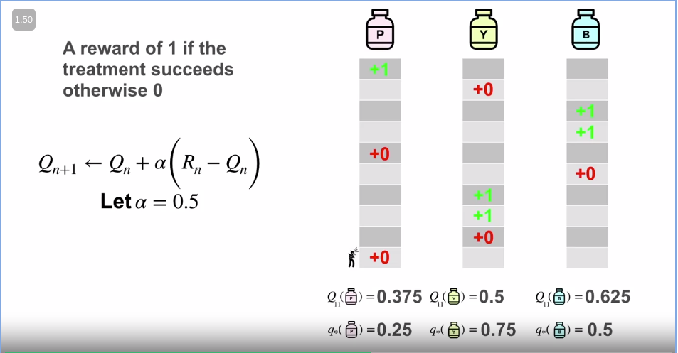
Let’s assume for the medical trial of the three medicines, the optimum action values are $q_1 = 0.25, q_2=0.75, and q_3=0.5$ respectively.

But initially, we do not know them of course! How about we start with high initial values?

$Q_1 = Q_2 = Q_3 = 2$

From the incremental update equation,

$Q_{n+1} $←$ Q_n + \alpha(R_n - Q_n)$

Let’s assume the positive feedback has point $1$ and the negative has $0$. After running some trials, we might get closer to the optimum values!

Comparison

So which approach is better? If we check the comparison plot

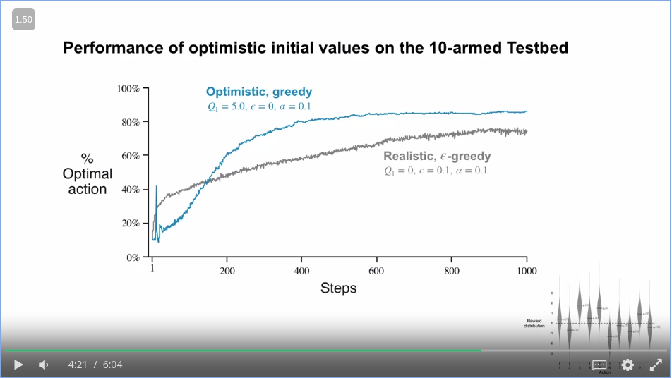
from the image above it seems that the optimistic initial value setting will help us more compared to the epsilon greedy!

Demerits

• We do not know what is the best optimistic initial value.
• It is temporary, i.e. after the first initial trials the explorations will get stopped

My thoughts

• We can use both epsilon greedy and optimistic initial values!

Another solution: Uppder confidence Action selection

The Epsilon greedy action selection works the following way

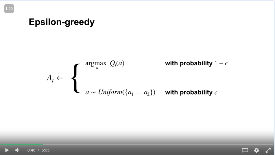
In this approach, we are choosing random actions with a uniform probability distribution. The problem is, we are giving the same weight to all of the random actions. How about while choosing the random action, we can choose the less explored action more? In other words, we prioritize the actions with less uncertainty (due to that action being less explored)!

For example, the uncertainty can be shown as follows,

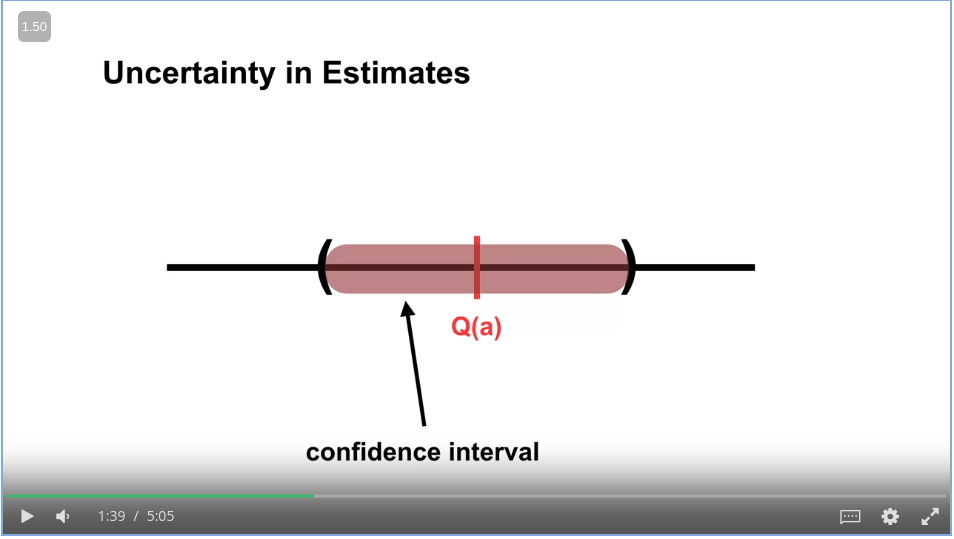
For this approach named Upper Confidence Bound selection aka UCB, we guess that the unknown action is good. i.e. with a high Q value.

The best part of the UCB equation is: It combines the exploration and the exploitation in one single equation!!

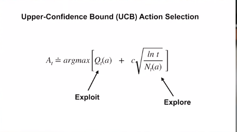
Where, - $t$ is the timesteps - $N_t(a)$ means the number of times an action $a$ is being taken. It means that the more we explore an action $a$, the lesser it will have an effect. Like the following example,

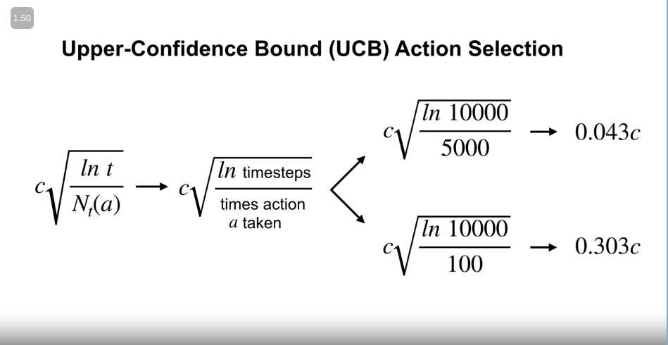
Where $c$ is the hyperparameter. on the 10-arm bandit test bed, the performance is as follows,

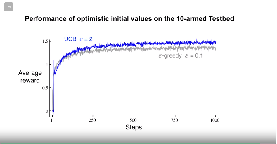
From the above plot, we can conclude that the UCB is performing better compared to the Epsilon greedy, despite its initial worse performance.

Conclusion

In this post, I wanted to describe my thoughts and understanding of the video of Reinforcement Learning Course 1 Week 1. Here, we explored the key concepts of Reinforcement learning. It took me a long time to write due to my work schedule. I hope the readers will be patient enough for the Week 2 posts. Till then, for any comments/questions, please contact me by email: sezan92[at]gmail[dot]com or by linkedin!

Reference

• All of the screenshots are from Course 1, Week 1 of Reinforcement Learning Specialization.