The Game, is On! REINFORCE!
Enter the world of Policy Gradient methods!
Video
First, let’s look at the resulting video, to understand what we are doing.
Episode 100 Trial

Episode 700 Trial

Episode 800 Trial
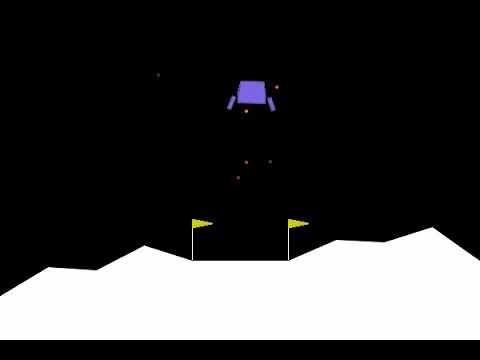
Have you wondered why, After episode 100 the agent was not working at all, and ad 700 it looks to learn the behavior and then at 800 it was stuck in the air? Let’s start!
Let’s look at the previous blogs
Previous blogs were about value-gradient methods where the actions were discrete. How about continuous actions? How about directly updating policy instead of choosing policy based on value function approximation? Here comes the world of Policy gradient methods!
Reinforce
In this blog, i am writing about new type of Reinforcement learning (will be referred as RL) method; REINFORCE method.
History
This method was first introduced by Ronald J. Williams in the Paper link. This paper is a lot more mathematical. Luckily we have intuition of it as well! More on that later.
Why Policy Gradient methods?
In the value-based methods the policies are not learned directly. The learning is done according to the value. The value function is continuously updated. WHAT IF WE value function is not neede? What if we want to learn the policy directly? Good or bad this is actually the reason. Value-based methods work well, if the policy is discrete. If the policy is discrete we can know which action to take based on value function. But if it is continuous, then that is impossible. One can discretize the actions, but again, how many actions can one take?
We don’t know which policy is the best!
Also, there is no way to explore different actions! If the actions is from -1.0 to 1.0, how can one explore the action , let’s say, 0.666 ? Here comes policy gradient methods!
Choice of actions Value-based methods choose actions randomly. Making action choice erratic, at least in the exploration stage. While Policy gradients do not have this problem. Actions are based on gradients!
Let’s talk about intuition
I find this blog to have the best intuition on Policy gradient method. Please check it out first before proceeding! I plan to write intuition blog in future.
Now it’s time of Code Walkthrough
How to run?
The repository is here
Assuming you have read the intuition blog, please go through the walkthrough.
Build Image
docker compose build
Run the container
docker compose up
Training with saving the video after every certain episode
python3 /src/reinforce_discrete.py LunarLander-v2 --train --save_model_path </path/to/save/the/model> --gamma <gamma hyper-parameter> --epoch <num_of_epoch> --plot <to plot or not> --plot_fig_path </path/to/save/the/plot> --train_video_dir </path/to/train_video> --train_video_every <number_of_episodes_to_save_video>
Inference
-
To setup for inference, run from outside the docker container
sudo xhost +SI:localuser:<username> -
From another terminal run
docker exec -it <container_name>and inside the container run,python3 /src/reinforce_discrete.py LunarLander-v2 --infer --infer_weight /path/to/saved/weight --infer_render <to render the inference or not> --infer_render_fps <fps for render video> --infer_video </path/to/save/inference/rendered/video.>
What about the codebase?
Policy Script
The __init__ and forward methods are same to previous blogs. A simple neural network of 2 hidden layers.
class Policy:

    def __init__(self, s_size=4, fc1_size=150, fc2_size=120, a_size=2):
            super(Policy, self).__init__()
            self.fc1 = nn.Linear(s_size, fc1_size)
            self.fc2 = nn.Linear(fc1_size, fc2_size)
            self.final = nn.Linear(fc2_size, a_size)

    def forward(self, x):
            x = F.relu(self.fc1(x))
            x = F.relu(self.fc2(x))
            x = self.final(x)
            return F.softmax(x, dim=1)
- But the Action is a bit different this time!
    def act(self, state):
        state = torch.from_numpy(state).float().unsqueeze(0).to(device)
        probs = self.forward(state).cpu()
        m = Categorical(probs)
        action = m.sample()
        return action.item(), m.log_prob(action)
-
So we see that the
actmethod outputs the action value (obvious) and the action probability. -
Why probability ? The reason is because for the gradient ascent we will need the action probability. If we look at the equation for gradient ascent,
\[\nabla_\theta J(\theta)= \hat{A}(s,a)\nabla_\theta\log\pi_{\theta}(s|a)\] \[\theta = \theta + \alpha\nabla_\theta J(\theta)\]So it turns out, we need to have action value to run the agent and the log probability as well.
rl/rl/renforce.py script
-
Function definition
def reinforce_discrete( env, policy, model_weights_path, n_episodes=1000, max_t=1000, gamma=1.0, print_every=100, learning_rate=1e-2 ): scores = [] -
make an optimizer
optimizer = optim.Adam(policy.parameters(), lr=learning_rate) -
Get the action and log probability, get the reward, and save the rewards with log probability
for i_episode in range(1, n_episodes + 1): saved_log_probs = [] rewards = [] state = env.reset() states = [state] for t in range(max_t): action, log_prob = policy.act(state) saved_log_probs.append(log_prob) state, reward, done, _ = env.step(action) rewards.append(reward) states.append(state) if done: break scores.append(sum(rewards)) -
We will get expected rewards based on gamma. It is the application of the following equation,
\[E = R_i + \gamma R_{i +1} + \gamma^2R_{i+2} ....\gamma^{n-1}R_{i + n - 1}\]expected_rewards = get_expected_reward(rewards, gamma) state_values = get_state_values(rewards) policy_loss = [] -
Advantage according to the equation, get the policy loss and backpropagate.
Advantage is , as following \(A = E - mean(E)\) There is a good explanation of using Advantage here. But for now, it is enough to understand that, Advantage is more dependant on action by an agent, i.e. it shows the effect of taking an action for a certain state , and hence named Advantage maybe!
The code is as follows
          for i, log_prob in enumerate(saved_log_probs):
              A = expected_rewards[i] - np.mean(expected_rewards)
              policy_loss.append((-log_prob * A).float())
          policy_loss = torch.cat(policy_loss).sum()

          optimizer.zero_grad()
          policy_loss.backward()
          optimizer.step()

          if i_episode % print_every == 0:
              print(
                  "INFO: Episode {}\tAverage Score: {:.2f}".format(
                      i_episode, np.mean(scores[-print_every:])
                  )
              )
          if np.mean(scores[-print_every:]) >= 195.0:
              print(
                  "INFO: Environment solved in {:d} episodes!\tAverage Score: {:.2f}".format(
                      i_episode - 100, np.mean(scores[-print_every:])
                  )
              )
              break
      print(f"INFO: Saving the weights in {model_weights_path}")
      torch.save(policy.state_dict(), model_weights_path)
      return scores
Score plot
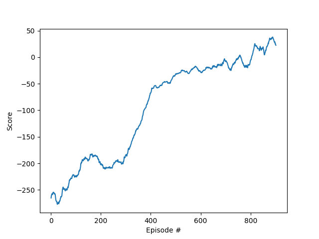
The score plots of the entire training is as follows.
Problem with this approach
If you check the plot above, and also the videos referred to at the beginning, you will notice that the agent is not stable enough. After 700 episodes, at the 800th episode, it should do the optimum task to sit down at the right place. But it was hovering, which can be referred to two cases
- This method only considers the reward due to action and no evaluation of the state! So when hovering it might be getting a higher reward than falling down. It is sub-optimal behavior only based on actions!
- Hence, the training process has a higher variance. As we are training the agent based only on the rewards of the actions, not on the value of the state.
- How to solve it? We will find out in the next blogs!
TODO
I was planning to compare the score plots! When I will be able to do it, I will update you!
- Compare Reinforce method plots to DQN based methods.
Conclusion
To conclude, Reinforce method opens the pathway to policy gradient methods, making continuous action based problems easier to solve. But it has high variance issue. It needs to be updated. Which will be subject to my upcoming blogs. Although I mentioned about the continuous actions, this blog is still working with discrete actions! In the part 2 of reinforce, I will try to update the action into Continuous one!
If you have any question or comment, please ask at sezan92[at]gmail[dot]com