Facial Keypoint Estimation

Facial Landmarks Estimation and features visualization github

Here, I am working on training a model to estimate facial keypoints. I was inspired by Udacitys Computer Vision Nanodegrees Project of Keypoint Detection. The difference is, I used Facial Keypoint Dataset used in a Kaggle Competition .

Loading the Dataset

The first step is to load the dataset. I took the help from this kaggle notebook

import numpy as np
import matplotlib.pyplot as plt
import pandas as pd
from IPython.display import clear_output
from time import sleep
import os
Train_Dir = 'training.csv'
train_data = pd.read_csv(Train_Dir)  

Lets have a look at the dataset

train_data.head(5)

	left_eye_center_x	left_eye_center_y	right_eye_center_x	right_eye_center_y	left_eye_inner_corner_x	left_eye_inner_corner_y	left_eye_outer_corner_x	left_eye_outer_corner_y	right_eye_inner_corner_x	right_eye_inner_corner_y	...	nose_tip_y	mouth_left_corner_x	mouth_left_corner_y	mouth_right_corner_x	mouth_right_corner_y	mouth_center_top_lip_x	mouth_center_top_lip_y	mouth_center_bottom_lip_x	mouth_center_bottom_lip_y	Image
0	66.033564	39.002274	30.227008	36.421678	59.582075	39.647423	73.130346	39.969997	36.356571	37.389402	...	57.066803	61.195308	79.970165	28.614496	77.388992	43.312602	72.935459	43.130707	84.485774	238 236 237 238 240 240 239 241 241 243 240 23...
1	64.332936	34.970077	29.949277	33.448715	58.856170	35.274349	70.722723	36.187166	36.034723	34.361532	...	55.660936	56.421447	76.352000	35.122383	76.047660	46.684596	70.266553	45.467915	85.480170	219 215 204 196 204 211 212 200 180 168 178 19...
2	65.057053	34.909642	30.903789	34.909642	59.412000	36.320968	70.984421	36.320968	37.678105	36.320968	...	53.538947	60.822947	73.014316	33.726316	72.732000	47.274947	70.191789	47.274947	78.659368	144 142 159 180 188 188 184 180 167 132 84 59 ...
3	65.225739	37.261774	32.023096	37.261774	60.003339	39.127179	72.314713	38.380967	37.618643	38.754115	...	54.166539	65.598887	72.703722	37.245496	74.195478	50.303165	70.091687	51.561183	78.268383	193 192 193 194 194 194 193 192 168 111 50 12 ...
4	66.725301	39.621261	32.244810	38.042032	58.565890	39.621261	72.515926	39.884466	36.982380	39.094852	...	64.889521	60.671411	77.523239	31.191755	76.997301	44.962748	73.707387	44.227141	86.871166	147 148 160 196 215 214 216 217 219 220 206 18...

5 rows × 31 columns

Its a bit big. Lets look at the column names

train_data.columns

Index(['left_eye_center_x', 'left_eye_center_y', 'right_eye_center_x',
       'right_eye_center_y', 'left_eye_inner_corner_x',
       'left_eye_inner_corner_y', 'left_eye_outer_corner_x',
       'left_eye_outer_corner_y', 'right_eye_inner_corner_x',
       'right_eye_inner_corner_y', 'right_eye_outer_corner_x',
       'right_eye_outer_corner_y', 'left_eyebrow_inner_end_x',
       'left_eyebrow_inner_end_y', 'left_eyebrow_outer_end_x',
       'left_eyebrow_outer_end_y', 'right_eyebrow_inner_end_x',
       'right_eyebrow_inner_end_y', 'right_eyebrow_outer_end_x',
       'right_eyebrow_outer_end_y', 'nose_tip_x', 'nose_tip_y',
       'mouth_left_corner_x', 'mouth_left_corner_y', 'mouth_right_corner_x',
       'mouth_right_corner_y', 'mouth_center_top_lip_x',
       'mouth_center_top_lip_y', 'mouth_center_bottom_lip_x',
       'mouth_center_bottom_lip_y', 'Image'],
      dtype='object')

We see, the columns are the name of the facial landmarks , and the last column is the image data

So we need to seperate and preprocess the image and facial landmarks

Lets check if there are any null values

train_data.isnull().any().value_counts()

True     28
False     3
dtype: int64

There are 28 null values

train_data.fillna(method = 'ffill',inplace = True)
#train_data.reset_index(drop = True,inplace = True

Lets collect all the images in one list

imag = []
for i in range(0,train_data.shape[0]):
    img = train_data['Image'][i].split(' ')
    img = np.array(['0' if x == '' else x for x in img])
    img = img.reshape(-1,96,96,1)
    imag.append(img)

image_list = np.array(imag,dtype = 'float')
X_train = image_list.reshape(-1,96,96,1)

Lets plot one image

plt.imshow(X_train[100].reshape(96,96),cmap='gray')
plt.show()

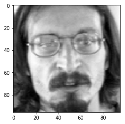
Done!

Lets get the keypoints

training = train_data.drop('Image',axis = 1)

y_train = []
for i in range(0,7049):
    y = training.iloc[i,:]

    y_train.append(y)
y_train = np.array(y_train,dtype = 'float')

Lets do the same process for test data

Test_Dir = 'test.csv'
test_data = pd.read_csv(Test_Dir)
test_data.fillna(method = 'ffill',inplace = True)
#train_data.reset_index(drop = True,inplace = True

imag = []
for i in range(0,test_data.shape[0]):
    img = test_data['Image'][i].split(' ')
    img = np.array(['0' if x == '' else x for x in img])
    img = img.reshape(-1,96,96,1)
    imag.append(img)
    
X_test = np.array(imag)
print("before")
print(X_test.shape)

X_test = X_test.reshape(-1,96,96,1)
print("After")
print(X_test.shape)

before
(1783, 1, 96, 96, 1)
After
(1783, 96, 96, 1)

Lets save the images in to a pickle file

import pickle

pickle.dump(X_train,open("train_images.pkl","wb"))
pickle.dump(y_train,open("train_labels.pkl","wb"))
pickle.dump(X_test,open("test_images.pkl","wb"))

Visualize Image

We have to visualize the image with the facial landmarks

X_train = pickle.load(open("train_images.pkl","rb"))
y_train = pickle.load(open("train_labels.pkl","rb"))

Lets take a sample image

image= X_train[1717]

label= y_train[1717]

label

array([63.69583007, 41.80198701, 32.86046701, 40.41980434, 58.26235236,
       42.3298851 , 69.9596772 , 42.43179593, 38.25399567, 40.92324383,
       26.98347338, 40.03458141, 56.14862342, 33.55158196, 77.60328461,
       33.42403661, 47.8555892 , 27.91678736, 19.25751152, 24.33053325,
       39.98793743, 59.92543854, 59.81812037, 79.77184453, 31.19594436,
       79.75499805, 44.58350812, 79.22635539, 44.33620174, 81.42279995])

A function to visualize the image with label

def visualize(image,label):
    x,y=[],[]
    for i in range(label.shape[0]):
        if (i+1)%2==1:
            x.append(label[i])
        else:
            y.append(label[i])


    plt.imshow(image.reshape(96,96),cmap="gray")
    plt.scatter(x,y,c="r")

visualize(image,label)

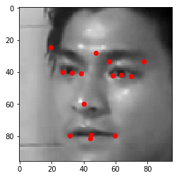
Awesome!! Let start Neural Network!!

Training

Importing necessary packages

import torch
from torch.autograd import Variable
import torch.nn as nn
import torch.nn.functional as F

Fixing the random seed

SEED=1001

torch.manual_seed(SEED)
np.random.seed(SEED)

Some Hyperparameters

BATCH_SIZE=128

EPOCHS=100

Here , I defined a simple four layer Convolutional neural network. It is just for baseline model. My intention was to to make a full pipeline first and then increase the complexity if necessary . Also to visualize the layers if they really can extract the features.

Model

The problem is a regression problem. It detects the x,y coordinates of 15 keypoints. Hence the output size is (30,).

class SezanNet(nn.Module):
    def __init__(self):
        super(SezanNet, self).__init__()
        self.conv1 = nn.Conv2d(in_channels=1, out_channels=32, kernel_size=(4, 4),stride=2) ## 32x47x47
        self.dropout=nn.Dropout()
        self.conv2 = nn.Conv2d(in_channels=32, out_channels=64, kernel_size=(4, 4),stride=2) # 64x22x22
        self.conv3 = nn.Conv2d(in_channels=64,out_channels=128,kernel_size=(3,3),stride=2) # 128x10x10
        self.conv4 = nn.Conv2d(in_channels=128,out_channels=256,kernel_size=(1,1),stride=2) # 256x5x5
        
        self.relu = nn.ReLU()
        self.fc1 = nn.Linear(in_features=256*5*5,out_features=30)
        
    def forward(self,x):
        x = self.dropout(self.relu(self.conv1(x)))
        x = self.dropout(self.relu(self.conv2(x)))
        x = self.dropout(self.relu(self.conv3(x)))
        x = self.dropout(self.relu(self.conv4(x)))
        x = x.view(x.size(0),-1)
        x = self.fc1(x)
        return x
        

net = SezanNet()

Importing Data

But Hold on!

I got this idea ( actually i copied from Computer Vision Nanodegree) , of making a seperate script data_load.py only for data loading. I am not showing the full process . But it is sufficient to say that , the script has three classes

• Normalize it normalizes the image from 0.0 to 1.0 and keypoints from -1.0 to 1.0
• Totensor it converts images as well keypoints to pytorch tensor
• FacialKeypointsDataset - it takes the images and labels pickle files and transforms them all according to transform classes.

You can get some examples here

from data_load import *

train_data_transform = transforms.Compose([Normalize(), \
                                           ToTensor()])

dataset = FacialKeypointsDataset("train_images.pkl","train_labels.pkl",transform=train_data_transform)

Splitting to train and test result

from sklearn.model_selection import train_test_split

train_data,val_data=train_test_split(dataset,test_size=0.2)

Dataloader generator

from torch.utils.data import Dataset, DataLoader

train_loader=DataLoader(train_data,batch_size=BATCH_SIZE,shuffle=True)

validation_loader= DataLoader(val_data,batch_size=BATCH_SIZE,shuffle=True)

from torch.autograd import Variable

import torch.optim as optim

criterion = nn.MSELoss()

optimizer = optim.Adam(net.parameters(), lr=0.001)

Training

losses=[]
validation_losses=[]
for epoch in range(EPOCHS):
    loss_sum=0
    val_loss_sum=0
    net.train()
    for iteration_train,batch_data in enumerate(train_loader):
        images=batch_data["image"]
        keypoints=batch_data["keypoints"]
        images= Variable(images)
        keypoints=Variable(keypoints)
        images=images.float()
        keypoints=keypoints.float()
        output_keypoints=net(images)
        loss = torch.sqrt(criterion(keypoints, output_keypoints))
        optimizer.zero_grad()
        loss_sum+=loss.data[0]
        loss.backward()
        optimizer.step()
    net.eval()
    for iteration_val,batch_data in enumerate(validation_loader):
        images=batch_data["image"]
        keypoints=batch_data["keypoints"]
        images= Variable(images)
        keypoints=Variable(keypoints)
        images=images.float()
        keypoints=keypoints.float()
        output_keypoints=net(images)
        loss = torch.sqrt(criterion(keypoints, output_keypoints))
        val_loss_sum+=loss.data[0]
        
    
    print("train loss {} , validation loss {}".format(loss_sum/(iteration_train+1),val_loss_sum/(iteration_val+1)))
    losses.append(loss_sum/(iteration_train+1))
    validation_losses.append(val_loss_sum/(iteration_val+1))

/usr/local/lib/python3.6/site-packages/ipykernel_launcher.py:17: UserWarning: invalid index of a 0-dim tensor. This will be an error in PyTorch 0.5. Use tensor.item() to convert a 0-dim tensor to a Python number
/usr/local/lib/python3.6/site-packages/ipykernel_launcher.py:30: UserWarning: invalid index of a 0-dim tensor. This will be an error in PyTorch 0.5. Use tensor.item() to convert a 0-dim tensor to a Python number


train loss 5.425237655639648 , validation loss 3.8939077854156494
train loss 3.9826440811157227 , validation loss 3.7200019359588623
train loss 3.9659817218780518 , validation loss 3.7740650177001953
train loss 3.9442718029022217 , validation loss 3.808095932006836
train loss 3.922896385192871 , validation loss 3.700185775756836
train loss 3.8800809383392334 , validation loss 3.7662575244903564
train loss 3.8388638496398926 , validation loss 3.619922637939453
train loss 3.7563650608062744 , validation loss 3.506974935531616
train loss 3.6804325580596924 , validation loss 3.4494895935058594
train loss 3.622939348220825 , validation loss 3.35968279838562
train loss 3.537247657775879 , validation loss 3.3125455379486084
train loss 3.4457898139953613 , validation loss 3.2589786052703857
train loss 3.383971929550171 , validation loss 3.0803232192993164
train loss 3.3441357612609863 , validation loss 3.04178786277771
train loss 3.319330930709839 , validation loss 3.076205253601074
train loss 3.2813069820404053 , validation loss 3.0077173709869385
train loss 3.265842914581299 , validation loss 3.2337818145751953
train loss 3.2375996112823486 , validation loss 3.0629327297210693
train loss 3.208923578262329 , validation loss 3.0416555404663086
train loss 3.1732380390167236 , validation loss 2.9472620487213135
train loss 3.157954216003418 , validation loss 2.949187994003296
train loss 3.1411375999450684 , validation loss 2.9549710750579834
train loss 3.1253421306610107 , validation loss 2.927802324295044
train loss 3.1084532737731934 , validation loss 3.0862462520599365
train loss 3.1061744689941406 , validation loss 2.975170850753784
train loss 3.106091022491455 , validation loss 2.856614112854004
train loss 3.0634639263153076 , validation loss 3.016416549682617
train loss 3.0432448387145996 , validation loss 2.933286428451538
train loss 3.030418872833252 , validation loss 2.877021551132202
train loss 3.0282084941864014 , validation loss 2.8490371704101562
train loss 3.0325286388397217 , validation loss 2.853555679321289
train loss 3.0381109714508057 , validation loss 3.0146563053131104
train loss 3.016242027282715 , validation loss 2.7567574977874756
train loss 3.0050241947174072 , validation loss 2.895277261734009
train loss 2.988123893737793 , validation loss 2.8342654705047607
train loss 2.9882636070251465 , validation loss 2.7939417362213135
train loss 2.9727416038513184 , validation loss 2.9796302318573
train loss 2.9797611236572266 , validation loss 2.7760326862335205
train loss 2.9760663509368896 , validation loss 2.8358542919158936
train loss 2.9660208225250244 , validation loss 2.8890163898468018
train loss 2.9585134983062744 , validation loss 2.896223783493042
train loss 2.9499399662017822 , validation loss 2.7742865085601807
train loss 2.9291110038757324 , validation loss 2.7883126735687256
train loss 2.9365837574005127 , validation loss 3.0206029415130615
train loss 2.9413442611694336 , validation loss 2.809206247329712
train loss 2.9380855560302734 , validation loss 2.7912709712982178
train loss 2.9286677837371826 , validation loss 2.7881956100463867
train loss 2.9188692569732666 , validation loss 2.8298656940460205
train loss 2.915041446685791 , validation loss 2.7835710048675537
train loss 2.898670196533203 , validation loss 2.717679977416992
train loss 2.891162395477295 , validation loss 2.7501237392425537
train loss 2.891622543334961 , validation loss 2.7899935245513916
train loss 2.8966169357299805 , validation loss 2.8692080974578857
train loss 2.881467580795288 , validation loss 2.836939811706543
train loss 2.8737008571624756 , validation loss 2.8376893997192383
train loss 2.8766493797302246 , validation loss 2.8025715351104736
train loss 2.851918935775757 , validation loss 2.707432508468628
train loss 2.8505139350891113 , validation loss 2.8986942768096924
train loss 2.8560967445373535 , validation loss 2.7655723094940186
train loss 2.829793930053711 , validation loss 2.9476335048675537
train loss 2.850368022918701 , validation loss 2.829697370529175
train loss 2.858083486557007 , validation loss 2.776062250137329
train loss 2.8635566234588623 , validation loss 2.7491672039031982
train loss 2.848045825958252 , validation loss 2.712719678878784
train loss 2.843352794647217 , validation loss 2.7817611694335938
train loss 2.825275421142578 , validation loss 2.713456869125366
train loss 2.8239686489105225 , validation loss 2.689215660095215
train loss 2.812502145767212 , validation loss 2.7039153575897217
train loss 2.815408229827881 , validation loss 2.858944892883301
train loss 2.817307710647583 , validation loss 3.0894386768341064
train loss 2.830634355545044 , validation loss 2.6975975036621094
train loss 2.8166542053222656 , validation loss 2.802992582321167
train loss 2.803333282470703 , validation loss 2.751505136489868
train loss 2.785895347595215 , validation loss 2.9604785442352295
train loss 2.788135290145874 , validation loss 2.723773717880249
train loss 2.785355567932129 , validation loss 2.6629910469055176
train loss 2.7883992195129395 , validation loss 2.6921465396881104
train loss 2.7980244159698486 , validation loss 2.6780617237091064
train loss 2.7924506664276123 , validation loss 2.7146503925323486
train loss 2.756983518600464 , validation loss 2.7129361629486084
train loss 2.779189109802246 , validation loss 2.669135093688965
train loss 2.7842793464660645 , validation loss 2.821007013320923
train loss 2.7794337272644043 , validation loss 2.706434965133667
train loss 2.750030994415283 , validation loss 2.746302366256714
train loss 2.7764477729797363 , validation loss 2.6850740909576416
train loss 2.756556749343872 , validation loss 2.687755584716797
train loss 2.760605812072754 , validation loss 2.805509567260742
train loss 2.761059045791626 , validation loss 2.6881396770477295
train loss 2.753006935119629 , validation loss 2.763848304748535
train loss 2.740943193435669 , validation loss 2.7135117053985596
train loss 2.7341177463531494 , validation loss 2.8102972507476807
train loss 2.7550344467163086 , validation loss 2.6504886150360107
train loss 2.7519311904907227 , validation loss 2.9423024654388428
train loss 2.7594923973083496 , validation loss 2.6570122241973877
train loss 2.751809597015381 , validation loss 2.7266156673431396
train loss 2.7333316802978516 , validation loss 2.806152105331421
train loss 2.7397658824920654 , validation loss 2.7984392642974854
train loss 2.726048469543457 , validation loss 2.7089881896972656
train loss 2.7385780811309814 , validation loss 2.7740771770477295
train loss 2.7270455360412598 , validation loss 2.7067394256591797

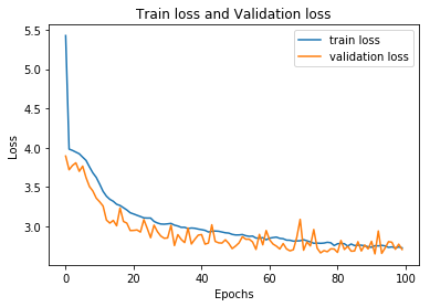
plt.plot(losses,label="train loss")
plt.plot(validation_losses,label="validation loss")
plt.title("Train loss and Validation loss")
plt.xlabel("Epochs")
plt.ylabel("Loss")
plt.legend()

<matplotlib.legend.Legend at 0x7f124f15b588>

Test a sample

sample=val_data[454]

image=sample["image"].data.numpy()
keypoints=sample["keypoints"].data.numpy()

keypoints = keypoints*48+48

visualize(image,keypoints)

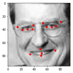
Prediction

image_tensor=torch.from_numpy(image.reshape(-1,1,96,96)).float()
net.eval()
predicted_keypoints=net(image_tensor)

predicted_keypoints=predicted_keypoints*48+48

predicted_keypoints=predicted_keypoints.data.numpy()

visualize(image,predicted_keypoints[0])

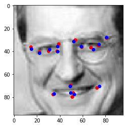
Lets make a function to visualize both prediction and actual keypoints

def visualize(image,label,prediction):
    x,y,x_pred,y_pred=[],[],[],[]
    for i in range(label.shape[0]):
        if (i+1)%2==1:
            x.append(label[i])
        else:
            y.append(label[i])
    for i in range(prediction.shape[0]):
        if (i+1)%2==1:
            x_pred.append(prediction[i])
        else:
            y_pred.append(prediction[i])


    plt.imshow(image.reshape(96,96),cmap="gray")
    plt.scatter(x,y,c="r")
    plt.scatter(x_pred,y_pred,c="b")

visualize(image,keypoints,predicted_keypoints[0])

Saving the model

torch.save(net.state_dict(),"network_state_dict.pkl")

Visualize the feature!

Another thing, I learned from the nanodeegree project is the Feature visualization . i.e. to visualize the features captured by each layer. But I thought, what If I could do more! I thought about using GradCAM in keypoint detection!!!

What is Grad-cam?

For people like me , In simple terms, Gradcam is some lines of codes to show which features or parts of the images activates to a particular layer when you feed into it. The most famouse example is this following image

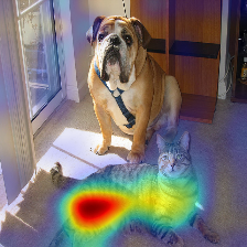
I used this repository for my purpose!. But Obviously, I made some changes!

Lets Go Grad-Cam!!

utility functions

import IPython

def imshow(img):
    _,ret = cv2.imencode('.jpg', img) 
    i = IPython.display.Image(data=ret)
    IPython.display.display(i)
    

def show_gradient(gradient):
    gradient = gradient.cpu().numpy().transpose(1, 2, 0)
    gradient -= gradient.min()
    gradient /= gradient.max()
    gradient *= 255.0
    plt.imshow(gradient.reshape(96,96),cmap="gray")


def show_gradcam(gcam, raw_image, paper_cmap=True):
    gcam = gcam.cpu().numpy()
    cmap = cm.jet_r(gcam)[..., :3] * 255.0
    raw_image=raw_image*255.0
    #cmap = cmap.reshape(96,96)
    raw_image=raw_image.reshape(96,96,1)
    if paper_cmap:
        alpha = gcam[..., None]
        gcam = alpha * cmap + (1 - alpha) * raw_image
    else:
        gcam = (cmap.astype(np.float) + raw_image.astype(np.float)) / 2
    plt.imshow(gcam)

class _BaseWrapper(object):
    def __init__(self, model):
        super(_BaseWrapper, self).__init__()
        self.device = next(model.parameters()).device
        self.model = model
        self.handlers = []  # a set of hook function handlers

    def _encode_one_hot(self, ids):
        one_hot = torch.zeros_like(self.logits).to(self.device)
        one_hot.scatter_(1, ids, 1.0)
        return one_hot

    def forward(self, image):
        self.image_shape = image.shape[2:]
        self.logits = self.model(image)
        
        return self.logits   # ordered results

    def backward(self, ids):
        """
        Class-specific backpropagation
        """
        
        self.model.zero_grad()
        self.logits.backward(gradient=ids, retain_graph=True)

    def generate(self):
        raise NotImplementedError

    def remove_hook(self):
        """
        Remove all the forward/backward hook functions
        """
        for handle in self.handlers:
            handle.remove()

This is the parent class of all GradCam classes. I changed the forward method such that , it will not output one hot encoded outputs! Why? . Because It is a regression problem , it doesnt need one hot encoded outputs!! So changed the line 17 to
return self.logits

Backpropagation Class

class BackPropagation(_BaseWrapper):
    def forward(self, image):
        self.image = image.requires_grad_()
        return super(BackPropagation, self).forward(self.image)

    def generate(self):
        gradient = self.image.grad.clone()
        self.image.grad.zero_()
        return gradient

bp = BackPropagation(model=net)
keypoints = bp.forward(image_tensor)  # sorted

bp.backward(ids=keypoints)
gradients = bp.generate()

show_gradient(gradients[0])

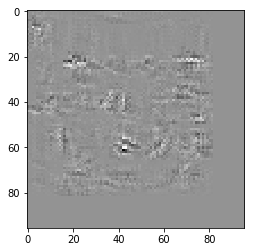
I dont think we can get some intuition from this map!

Lets try GradCAM!

import matplotlib.cm as cm

class GradCAM(_BaseWrapper):
    """
    "Grad-CAM: Visual Explanations from Deep Networks via Gradient-based Localization"
    https://arxiv.org/pdf/1610.02391.pdf
    Look at Figure 2 on page 4
    """

    def __init__(self, model, candidate_layers=None):
        super(GradCAM, self).__init__(model)
        self.fmap_pool = {}
        self.grad_pool = {}
        self.candidate_layers = candidate_layers  # list

        def save_fmaps(key):
            def forward_hook(module, input, output):
                self.fmap_pool[key] = output.detach()

            return forward_hook

        def save_grads(key):
            def backward_hook(module, grad_in, grad_out):
                self.grad_pool[key] = grad_out[0].detach()

            return backward_hook

        # If any candidates are not specified, the hook is registered to all the layers.
        for name, module in self.model.named_modules():
            if self.candidate_layers is None or name in self.candidate_layers:
                self.handlers.append(module.register_forward_hook(save_fmaps(name)))
                self.handlers.append(module.register_backward_hook(save_grads(name)))

    def _find(self, pool, target_layer):
        if target_layer in pool.keys():
            return pool[target_layer]
        else:
            raise ValueError("Invalid layer name: {}".format(target_layer))

    def generate(self, target_layer):
        fmaps = self._find(self.fmap_pool, target_layer)
        grads = self._find(self.grad_pool, target_layer)
        weights = F.adaptive_avg_pool2d(grads, 1)

        gcam = torch.mul(fmaps, weights).sum(dim=1, keepdim=True)
        gcam = F.relu(gcam)
        gcam = F.interpolate(
            gcam, self.image_shape, mode="bilinear", align_corners=False
        )

        B, C, H, W = gcam.shape
        gcam = gcam.view(B, -1)
        gcam -= gcam.min(dim=1, keepdim=True)[0]
        gcam /= gcam.max(dim=1, keepdim=True)[0]
        gcam = gcam.view(B, C, H, W)

        return gcam

gcam = GradCAM(model=net)
_ = gcam.forward(image_tensor)
gcam.backward(keypoints)

for generate method we need a name for target layer

for name,module in net.named_modules():
    print(name)

conv1
dropout
conv2
conv3
conv4
relu
fc1

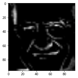
let’s check first layer conv1

regions = gcam.generate(target_layer="conv1")

Lets plot the generated region

gcam=regions[0,0].cpu().numpy()

plt.imshow(gcam,cmap="gray")

<matplotlib.image.AxesImage at 0x7f124d120fd0>

Lets get the colormap

cmap = cm.jet_r(gcam)[..., :3] 

result=(cmap.astype(np.float) + image.reshape(96,96,1).astype(np.float)) /2

plt.imshow(result,cmap="gray")

<matplotlib.image.AxesImage at 0x7f124d073b00>

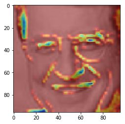
We see the keypoint areas or the areas adjacent to landmarks are activated! But there are other areas as well! Why them ? Most likely, using more robust network, will not activate them!